8 Introduction to R

For everyone that is more interested in all the topics I strongly recommend this eBook: R for Data Science

8.1 Getting started

Once you have started R, there are several ways to find help. First of all, (almost) every command is equipped with a help page that can be accessed via ?... (if the package is loaded). If the command is part of a package that is not loaded or you have no clue about the command itself, you can search the entire help (full-text) by using ??.... Be aware, that certain very-high level commands need to be put in quotation marks ?'function'. Many of the packages you find are either equipped with a demo() (get a list of all available demos using demo(package=.packages(all.available = TRUE))) and/or a vignette(), a document explaining the purpose of the package and demonstrating its work using suitable examples (find all available vignettes with vignette(package=.packages(all.available = TRUE))). If you want to learn how to do a certain task (e.g. conducting an event study vignette("eventstudies")²⁹).

Executing code in Rstudio is simple. Either you highlight the exact portion of the code that you want to execute and hit ctrl+enter, or you place the cursor just somewhere to execute this particular line of code with the same command.³⁰

8.2 Working directory

Before we start to learn how to program, we have to set a working directory. First, create a folder “researchmethods” (preferably never use directory names containing special characters or empty spaces) somewhere on citrix/your laptop, this will be your working directory where R looks for code, files to load and saves everything that is not designated by a full path (e.g. “D:/R/LAB/SS2018/…”). Note: In contrast to windows paths you have to use either “/” instead of “" or use two”\". Now set the working directory using setwd() and check with getwd()

setwd("D:/R/researchmethods")
getwd()

8.3 Basic calculations

3+5; 3-5; 3*5; 3/5
#> [1] 8
#> [1] -2
#> [1] 15
#> [1] 0.6
# More complex including brackets
(5+3-1)/(5*10)
#> [1] 0.14
# is different to 
5+3-1/5*10
#> [1] 6
# power of a variable
4*4*4
#> [1] 64
4^300
#> [1] 4.15e+180
# root of a variable
sqrt(16)
#> [1] 4
16^(1/2)
#> [1] 4
16^0.5
#> [1] 4
# exponential and logarithms
exp(3)
#> [1] 20.1
log(exp(3))
#> [1] 3
exp(1)
#> [1] 2.72
# Log to the basis of 2
log2(8)
#> [1] 3
2^log2(8)
#> [1] 8
# raise the number of digits shown
options(digits=6)
exp(1)
#> [1] 2.71828
# Rounding
20/3
#> [1] 6.66667
round(20/3,2)
#> [1] 6.67
floor(20/3)
#> [1] 6
ceiling(20/3)
#> [1] 7

8.4 Mapping variables

Defining variables (objects) in R is done via the arrow operator <- that works in both directions ->. Sometimes you will see someone use the equal sign = but for several (more complex) reasons, this is not advisable.

n <- 10
n
#> [1] 10
n <- 11
n
#> [1] 11
12 -> n
n
#> [1] 12
n <- n^2
n 
#> [1] 144

In the last case, we overwrite a variable recursively. You might want to do that for several reasons, but I advise you to rarely do that. The reason is that - depending on how often you have executed this part of the code already - n will have a different value. In addition, if you are checking the output of some calculation, it is not nice if one of the input variables always has a different value.

In a next step, we will check variables. This is a very important part of programming.

# check if m==10
m <- 11
m==10 # is equal to
#> [1] FALSE
m==11
#> [1] TRUE
m!=11 # is not equal to
#> [1] FALSE
m>10  # is larger than
#> [1] TRUE
m<10  # is smaller than
#> [1] FALSE
m<=11 # is smaller or equal than
#> [1] TRUE
m>=12 # is larger or equal than
#> [1] FALSE

If one wants to find out which variables are already set use ls(). Delete (Remove) variables using rm() (you sometimes might want to do that to save memory - in this case always follow the rm() command with gc()).

ls()  # list variables
#> [1] "EVAL"  "EVALf" "EVALt" "m"     "n"
rm(m) # remove m
ls()  # list variables again (m is missing)
#> [1] "EVAL"  "EVALf" "EVALt" "n"

Of course, often we do not only want to store numbers but also characters. In this case enclose the value by quotation marks: name <- "test". If you want to check whether a variable has a certain format use available commands starting with is.. If you want to change the format of a variable use as.

name <- "test"
is.numeric(n)
#> [1] TRUE
is.numeric(name)
#> [1] FALSE
is.character(n)
#> [1] FALSE
is.character(name)
#> [1] TRUE

If you do want to find out the format of a variable you can use class(). Slightly different information will be given by mode() and typeof()

class(n)
#> [1] "numeric"
class(name)
#> [1] "character"
mode(n)
#> [1] "numeric"
mode(name)
#> [1] "character"
typeof(n)
#> [1] "double"
typeof(name)
#> [1] "character"
# Lets change formats:
n1 <- n
is.character(n1)
#> [1] FALSE
n1 <- as.character(n)
is.character(n1)
#> [1] TRUE
as.numeric(name) # New thing: NA
#> Warning: NAs durch Umwandlung erzeugt
#> [1] NA

Before we learn about NA, we have to define logical variables that are very important when programming (e.g., as options in a function). Logical (boolean) variables will either assume TRUE or FALSE.

# last but not least we need boolean (logical) variables
n2 <- TRUE
is.numeric(n2)
#> [1] FALSE
class(n2)
#> [1] "logical"
is.logical(n2)
#> [1] TRUE
as.logical(2) # all values except 0 will be converted to TRUE
#> [1] TRUE
as.logical(0)
#> [1] FALSE

Now we can check whether a condition holds true. In this case, we check if m is equal to 10. The output (as you have seen before) is of type logical.

is.logical(n==10)
#> [1] TRUE
n3 <- n==10 # we can assign the logical output to a new variable
is.logical(n3)
#> [1] TRUE

Assignment: Create numeric variable x, set x equal to 5/3. What happens if you divide by 0? By Inf? Set y<-NA. What could this mean? Check if the variable is “na.” Is Inf numeric? Is NA numeric?

8.5 Sequences, vectors and matrices

In this chapter, we are going to learn about higher-dimensional objects (storing more information than just one number).

8.5.1 Sequences

We define sequences of elements (numbers/characters/logicals) via the concatenation operator c() and assign them to a variable. If one of the elements of a sequence is of type ‘character,’ the whole sequence will be converted to ‘character,’ else it will be of type ‘numeric’ (for other possibilities check the help ?vector). At the same type it will be of the type vector.

x <- c(1,3,5,6,7)
class(x)
#> [1] "numeric"
is.vector(x)
#> [1] TRUE
is.numeric(x)
#> [1] TRUE

To create ordered sequences make use of the command seq(from,to,by). Please note that often programmers are lazy and just write seq(1,10,2) instead of seq(from=1,to=10,by=2). However it makes code much harder to understand, can produce unintended results, and if a function is changed (which happens as R is always under construction) yield something very different to what was intended. Therefore I strongly encourage you to always specify the arguments of a function by name. To do this I advise you to make use of the tab a lot. Tab helps you to complete commands, produces a list of different commands starting with the same letters (if you do not completely remember the spelling for example), helps you to find out about the arguments and even gives information about the intended/possible values of the arguments. A nice way and shortcut for creating ordered/regular sequences with distance (by=) one is given by the : operator: 1:10 is equal to seq(from=1,to=10,by=1).

x1 <- seq(from=1,to=5,by=1)
x2 <- 1:5

One can operate with sequences in the same way as with numbers. Be aware of the order of the commands and use brackets where necessary!

1:10-1
#>  [1] 0 1 2 3 4 5 6 7 8 9
1:(10-1)
#> [1] 1 2 3 4 5 6 7 8 9
1:10^2-2 *3
#>   [1] -5 -4 -3 -2 -1  0  1  2  3  4  5  6  7  8  9 10 11 12 13 14 15 16 17 18 19
#>  [26] 20 21 22 23 24 25 26 27 28 29 30 31 32 33 34 35 36 37 38 39 40 41 42 43 44
#>  [51] 45 46 47 48 49 50 51 52 53 54 55 56 57 58 59 60 61 62 63 64 65 66 67 68 69
#>  [76] 70 71 72 73 74 75 76 77 78 79 80 81 82 83 84 85 86 87 88 89 90 91 92 93 94

Assignment: 1. Create a series from -1 to 5 with distances 0.5? Can you find another way to do it using the : operator and standard mathematical operations? 2. Create the same series, but this time using the “length”-option 3. Create 20 ones in a row (hint: find a function to do just that)

Of course, all logical operations are possible for vectors, too. In this case, the output is a vector of logicals having the same size as the input vector. You can check if a condition is true for any() or all() parts of the vector.

8.5.2 Random Sequences

One of the most important tasks of any programming language that is used for data analysis and research is the ability to generate random numbers. In R all the random number commands start with an r..., e.g. random normal numbers rnorm(). To find out more about the command use the help ?rnorm. All of these commands are a part of the stats package, where you find available commands using the package help: library(help=stats). Notice that whenever you generate random numbers, they are different. If you prefer to work with the same set of random numbers (e.g. for testing purposes) you can fix the starting value of the random number generator by setting the seed to a chosen number set.seed(123). Notice that you have to execute set.seed() every time before (re)using the random number generator.

rand1 <- rnorm(n = 100) # 100 standard normally distributed random numbers
set.seed(134) # fix the starting value of the random number generator (then it will always)
rand1a <- rnorm(n = 100)

Assignment: 1. Create a random sequence of 20 N(0,2)-distributed variables and assign it to the variable rand2. 2. Create a random sequence of 200 Uniform(-1,1) distributed variables and save to rand3. 3. What other distributions can you find in the stats package? 4. Use the functions mean and sd. Manipulate the random variables to have a different mean and standard deviation. Do you remember the normalization process (z-score)?

As in the last assignment you can use all the functions you learned about in statistics to calculate the mean(), the standard deviation sd(), skewness() and kurtosis() (the latter two after loading and installing the moments package). To install/load a package we use install.packages() (only once) and then load the package with require().

#install.packages("moments") # only once, no need to reinstall every time
library(moments)
#> 
#> Attache Paket: 'moments'
#> Die folgenden Objekte sind maskiert von 'package:PerformanceAnalytics':
#> 
#>     kurtosis, skewness
#> Die folgenden Objekte sind maskiert von 'package:timeDate':
#> 
#>     kurtosis, skewness
mean(rand1a)
#> [1] -0.113145
sd(rand1a)
#> [1] 1.12316
skewness(rand1a)
#> [1] 0.23882
kurtosis(rand1a)
#> [1] 2.2025
summary(rand1a)
#>    Min. 1st Qu.  Median    Mean 3rd Qu.    Max. 
#>  -2.137  -0.996  -0.161  -0.113   0.631   2.453

8.6 Vectors and matrices

We have created (random) sequences above and can determine their properties, such as their length(). We also know how to manipulate sequences through mathematical operations, such as +-*/^. If you want to calculate a vector product, R provides the %*% operator. In many cases (such as %*%) vectors behave like matrices, automating whether they should be row or column-vectors. However, to make this more explicit transform your vector into a matrix using as.matrix. Now, it has a dimension and the property matrix. You can transpose the matrix using t(), calculate its inverse using solve() and manipulate in any other way imaginable. To create matrices use matrix() and be careful about the available options!

x <- c(2,4,5,8,10,12)
length(x)
#> [1] 6
dim(x)
#> NULL
x^2/2-1
#> [1]  1.0  7.0 11.5 31.0 49.0 71.0
x %*% x # R automatically multiplies row and column vector
#>      [,1]
#> [1,]  353
is.vector(x)
#> [1] TRUE
y <- as.matrix(x)
is.matrix(y); is.matrix(x)
#> [1] TRUE
#> [1] FALSE
dim(y); dim(x)
#> [1] 6 1
#> NULL
t(y) %*% y
#>      [,1]
#> [1,]  353
y %*% t(y)
#>      [,1] [,2] [,3] [,4] [,5] [,6]
#> [1,]    4    8   10   16   20   24
#> [2,]    8   16   20   32   40   48
#> [3,]   10   20   25   40   50   60
#> [4,]   16   32   40   64   80   96
#> [5,]   20   40   50   80  100  120
#> [6,]   24   48   60   96  120  144
mat <- matrix(data = x,nrow = 2,ncol = 3, byrow = TRUE)
dim(mat); ncol(mat); nrow(mat)
#> [1] 2 3
#> [1] 3
#> [1] 2
mat2 <- matrix(c(1,2,3,4),2,2) # set a new (quadratic) matrix
mat2i <- solve(mat2)
mat2 %*% mat2i
#>      [,1] [,2]
#> [1,]    1    0
#> [2,]    0    1
mat2i %*% mat2
#>      [,1] [,2]
#> [1,]    1    0
#> [2,]    0    1

Assignment: 1. Create this matrix matrix(c(1,2,2,4),2,2) and try to calculate its inverse. What is the problem? Remember the determinant? Calculate using det(). What do you learn? 2. Create a 4x3 matrix of ones and/or zeros. Try to matrix-multiply with any of the vectors/matrices used before. 3. Try to add/subtract/multiply matrices, vectors and scalars.

A variety of special matrices is available, such as diagonal matrices using diag(). You can glue matrices together columnwise (cbind()) or rowwise (rbind()).

diag(3)
#>      [,1] [,2] [,3]
#> [1,]    1    0    0
#> [2,]    0    1    0
#> [3,]    0    0    1
diag(c(1,2,3,4))
#>      [,1] [,2] [,3] [,4]
#> [1,]    1    0    0    0
#> [2,]    0    2    0    0
#> [3,]    0    0    3    0
#> [4,]    0    0    0    4
mat4 <- matrix(0,3,3)
mat5 <- matrix(1,3,3)
cbind(mat4,mat5)
#>      [,1] [,2] [,3] [,4] [,5] [,6]
#> [1,]    0    0    0    1    1    1
#> [2,]    0    0    0    1    1    1
#> [3,]    0    0    0    1    1    1
rbind(mat4,mat5)
#>      [,1] [,2] [,3]
#> [1,]    0    0    0
#> [2,]    0    0    0
#> [3,]    0    0    0
#> [4,]    1    1    1
#> [5,]    1    1    1
#> [6,]    1    1    1

8.6.1 The indexing system

We can access the row/column elements of any object with at least one dimension using [].

########################################################
### 8) The INDEXING System
# We can access the single values of a vector/matrix
x[2] # one-dim
#> [1] 4
mat[,2] # two-dim column
#> [1]  4 10
mat[2,] # two-dim row
#> [1]  8 10 12
i <- c(1,3)
mat[i]
#> [1] 2 4
mat[1,2:3] # two-dim select second and third column, first row
#> [1] 4 5
mat[-1,] # two-dim suppress first row
#> [1]  8 10 12
mat[,-2] # two-dim suppress second column
#>      [,1] [,2]
#> [1,]    2    5
#> [2,]    8   12

Now we can use logical vectors/matrices to subset vectors/matrices. This is very useful for data mining.

mat>=5 # which elements are large or equal to 5?
#>       [,1]  [,2] [,3]
#> [1,] FALSE FALSE TRUE
#> [2,]  TRUE  TRUE TRUE
mat[mat>=5] # What are these elements?
#> [1]  8 10  5 12
which(mat>=5, arr.ind = TRUE) # another way with more explicit information
#>      row col
#> [1,]   2   1
#> [2,]   2   2
#> [3,]   1   3
#> [4,]   2   3

We can do something even more useful and name the rows and columns of a matrix usingcolnames() and rownames().

colnames(mat) <- c("a","b","c")
rownames(mat) <- c("A","B")
mat["A",c("b","c")]
#> b c 
#> 4 5

8.7 Functions in R

8.7.1 Useful Functions

Of course, there are thousands of functions available in R, especially through the use of packages. In the following you find a demo of the most useful ones.

x <- c(1,2,4,-1,2,8)  # example vector 1
x1 <- c(1,2,4,-1,2,8,NA,Inf) # example vector 2 (more complex)
sqrt(x) # square root of x
#> Warning in sqrt(x): NaNs wurden erzeugt
#> [1] 1.00000 1.41421 2.00000     NaN 1.41421 2.82843
x^3 # x to the power of ...
#> [1]   1   8  64  -1   8 512
sum(x) # sum of the elements of x
#> [1] 16
prod(x) # product of the elements of x
#> [1] -128
max(x) # maximum of the elements of x
#> [1] 8
min(x) # minimum of the elements of x
#> [1] -1
which.max(x) # returns the index of the greatest element of x
#> [1] 6
which.min(x) # returns the index of the smallest element of x
#> [1] 4
# statistical function - use rand1 and rand2 created before
range(x) # returns the minimum and maximum of the elements of x
#> [1] -1  8
mean(x) # mean of the elements of x
#> [1] 2.66667
median(x) # median of the elements of x
#> [1] 2
var(x) # variance of the elements of x
#> [1] 9.46667
sd(x) # standard deviation of the elements of x
#> [1] 3.07679
cov(x,x) # covariance between x and y
#> [1] 9.46667
cor(x,x) # linear correlation between x and y
#> [1] 1
# more complex functions
round(x, n) # rounds the elements of x to n decimals
#> [1]  1  2  4 -1  2  8
rev(x) # reverses the elements of x
#> [1]  8  2 -1  4  2  1
sort(x) # sorts the elements of x in increasing order
#> [1] -1  1  2  2  4  8
rank(x) # ranks of the elements of x
#> [1] 2.0 3.5 5.0 1.0 3.5 6.0
log(x) # computes natural logarithms of x
#> Warning in log(x): NaNs wurden erzeugt
#> [1] 0.000000 0.693147 1.386294      NaN 0.693147 2.079442
cumsum(x) # a vector which ith element is the sum from x[1] to x[i]
#> [1]  1  3  7  6  8 16
cumprod(x) # id. for the product
#> [1]    1    2    8   -8  -16 -128
cummin(x) # id. for the minimum
#> [1]  1  1  1 -1 -1 -1
cummax(x) # id. for the maximum
#> [1] 1 2 4 4 4 8
unique(x) # duplicate elements are suppressed
#> [1]  1  2  4 -1  8

8.7.2 More complex objects in R

Next to numbers, sequences/vectors and matrices R offers a variety of different and more complex objects that can stow more complex information than just numbers and characters (e.g. functions, output text. etc). The most important ones are data.frames (extended matrices) and lists. Check the examples below to see how to create these objects and how to access specific elements.

df <- data.frame(col1=c(2,3,4), col2=sin(c(2,3,4)), col3=c("a","b", "c"))
li <- list(x=c(2,3,4), y=sin(c(2,3,4)), z=c("a","b", "c","d","e"), fun=mean)
# to grab elements from a list or dataframe use $ or [[]]
df$col3; li$x # get variables
#> [1] "a" "b" "c"
#> [1] 2 3 4
df[,"col3"]; li[["x"]] # get specific elements that can also be numbered
#> [1] "a" "b" "c"
#> [1] 2 3 4
df[,3]; li[[1]]
#> [1] "a" "b" "c"
#> [1] 2 3 4

Assignment: 1. Get the second entry of element y of list x

8.7.3 Create simple functions in R

To create our own functions in R we need to give them a name, determine necessary input variables and whether these variables should be pre-specified or not. I use a couple of examples to show how to do this below.

?"function" # "function" is such a high-level object that it is interpreted before the "help"-command

# 1. Let's create a function that squares an entry x and name it square
square <- function(x){x^2}
square(5)
#> [1] 25
square(c(1,2,3))
#> [1] 1 4 9

# 2. Let us define a function that returns a list of several different results (statistics of a random vector v)
stats <- function(v){
  v.m <- mean(v) # create a variable that is only valid in the function
  v.sd <- sd(v)
  v.var <- var(v)
  v.output <- list(Mean=v.m, StandardDeviation=v.sd, Variance=v.var)
  return(v.output)
}
v <- rnorm(1000,mean=1,sd=5)
stats(v)
#> $Mean
#> [1] 0.962761
#> 
#> $StandardDeviation
#> [1] 4.81037
#> 
#> $Variance
#> [1] 23.1396
stats(v)$Mean
#> [1] 0.962761

# 3. A function can have standard arguments.
### This time we also create a random vector within the function and use its length as an input
stats2 <- function(n,m=0,s=1){
  v <- rnorm(n,mean=m,sd=s)
  v.m <- mean(v) # create a variable that is only valid in the function
  v.sd <- sd(v)
  v.var <- var(v)
  v.output <- list(Mean=v.m, StandardDeviation=v.sd, Variance=v.var)
  return(v.output)
}
stats2(1000000)
#> $Mean
#> [1] 0.000260415
#> 
#> $StandardDeviation
#> [1] 1.00077
#> 
#> $Variance
#> [1] 1.00154
stats2(1000,m=1)
#> $Mean
#> [1] 1.08296
#> 
#> $StandardDeviation
#> [1] 1.02642
#> 
#> $Variance
#> [1] 1.05354
stats2(1000,m=1,s=10)
#> $Mean
#> [1] 0.866102
#> 
#> $StandardDeviation
#> [1] 9.49228
#> 
#> $Variance
#> [1] 90.1034
stats2(m=1) # what happens if an obligatory argument is left out?
#> Error in rnorm(n, mean = m, sd = s): Argument "n" fehlt (ohne Standardwert)

Assignment: 1. Create a function that creates two random samples with length n and m from the normal and the uniform distribution resp., given the mean and sd for the first and min and max for the second distribution. The function shall then calculate the covariance-matrix and the correlation-matrix which it gives back in a named list.

8.8 Plotting

Plotting in R can be done very easily. Check the examples below to get a reference and idea about the plotting capabilities in R. A very good source for color names (that work in R) is (http://en.wikipedia.org/wiki/Web_colors).

?plot
?colors # very good source for colors: https://en.wikipedia.org/wiki/Web_colors

y1 <- rnorm(50,0,1)
plot(y1)
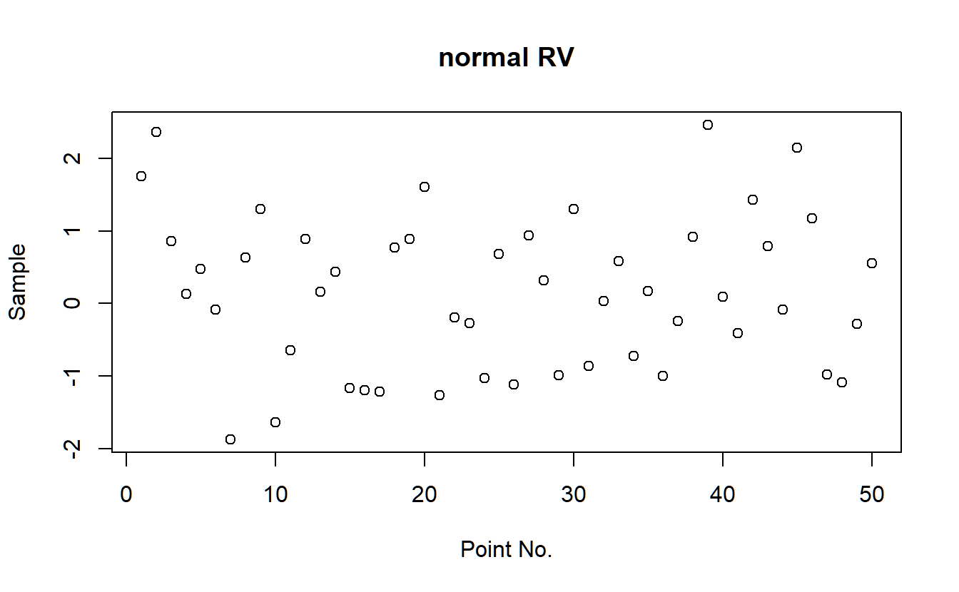
# set title, and x- and y-labels
plot(y1,main="normal RV",xlab="Point No.",ylab="Sample")
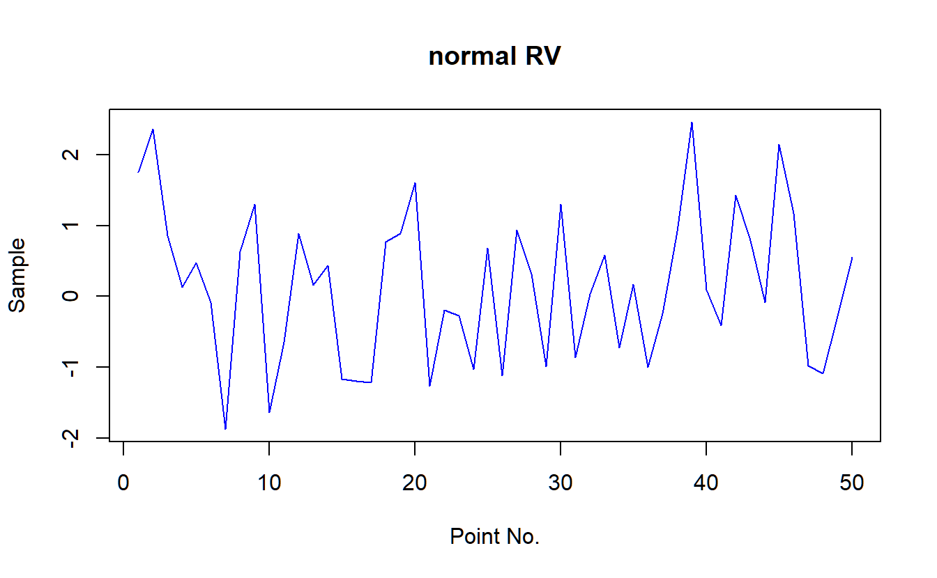
# now make a line between elements, and color everything blue
plot(y1,main="normal RV",xlab="Point No.",ylab="Sample",col="blue",type='l')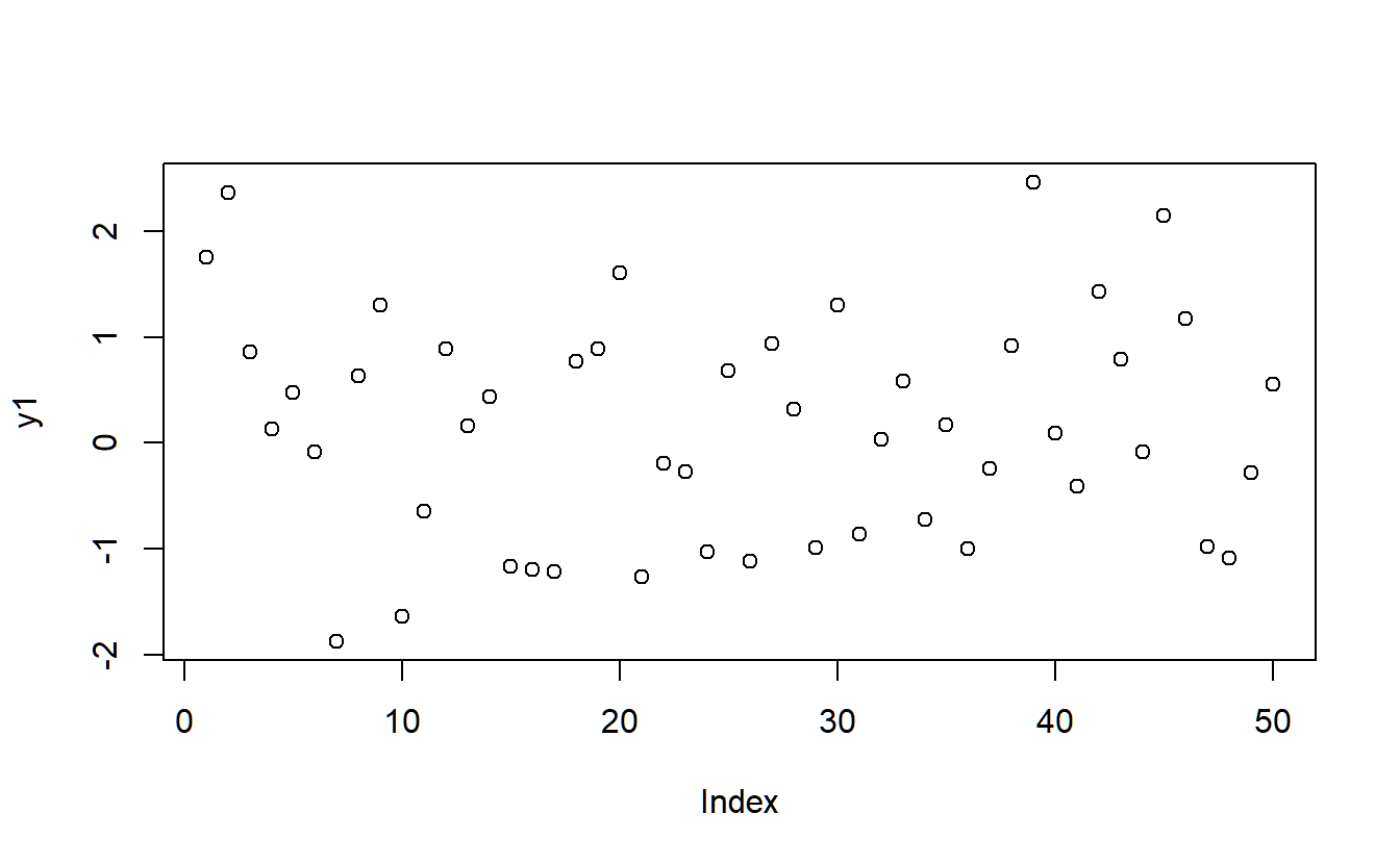

# if you want to save plots or open them in separate windows you can use x11, pdf, png, ...
?Devices
# x11 (opens seperate window)
x11(8,6)
plot(y1,main="normal RV",xlab="Point No.",ylab="Sample",col="blue",type='l')
# pdf
pdf("plot1.pdf",6,6)
plot(y1,main="normal RV",xlab="Point No.",ylab="Sample",col="blue",type='l',lty=2)
legend("topleft",col=c("blue"), lty=2, legend=c("normal Sample"))
dev.off()

# more extensive example
# X11(6,6)
par(mfrow=c(2,1),cex=0.9,mar=c(3,3,1,3)+0.1)
  plot(y1,main="normal RV",xlab="Point No.",ylab="Sample",col="blue",type='l',lty=2,ylim=c(-2.5,2.5),lwd=2)
  legend("topleft",col=c("blue"), lty=2, legend=c("normal Sample"))
  barplot(y1,col="blue") # making a barplot
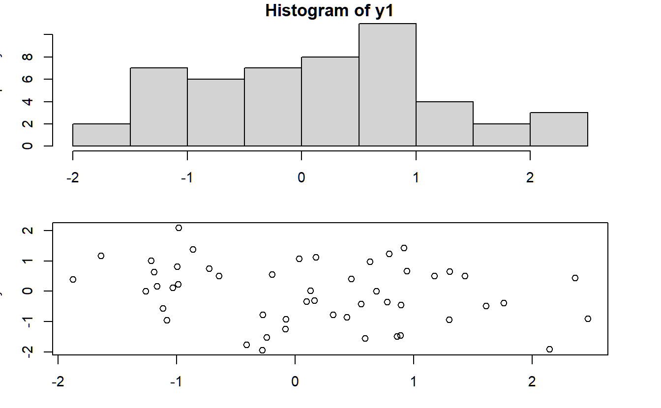
  # plotting a histogram
  hist(y1) # there is a nicer version available once we get to time series analysis
  # create a second sample
  y2 <- rnorm(50)
  # scatterplot
  plot(y1,y2)
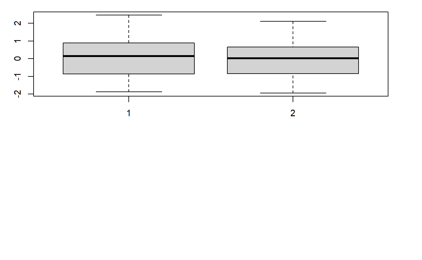
  # boxplot
  boxplot(y1,y2)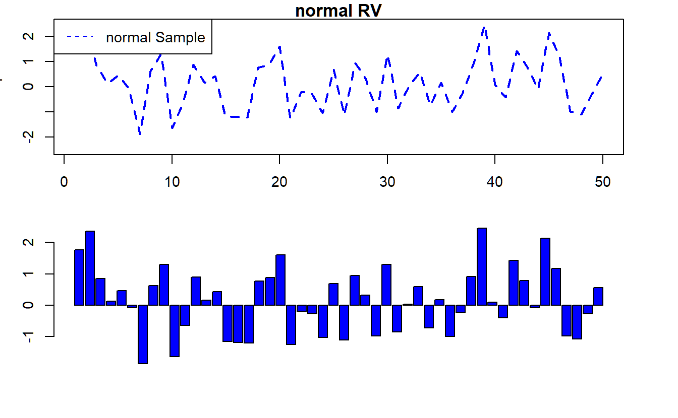

8.9 Control Structures

Last and least for this lecture we learn about control structure. These structures (for-loops, if/else checks etc) are very useful, if you want to translate a tedious manual task (e.g. in Excel) into something R should do for you and go step by step (e.g. column by column). Again, see below for a variety of examples and commands used in easy examples.

x <- sample(-15:15,10) # sample does draw randomly draw 10 numbers from the input vector -15:15
# 1. We square every element of vector x in a loop
y <- NULL # 1.a) set an empty variable (NULL means it is truly nothing and has no pre-specified dimension/length)
is.null(y)
#> [1] TRUE
# 1.b) Use an easy for-loop:
for (i in 1:length(x)){
  y[i] <- x[i]^2
}

# 2. Now we use an if-condition to only replace negative values
y <- NULL
for (i in 1:length(x)){
  y[i] <- x[i]
  if(x[i]<0) {y[i] <- x[i]^2}
}

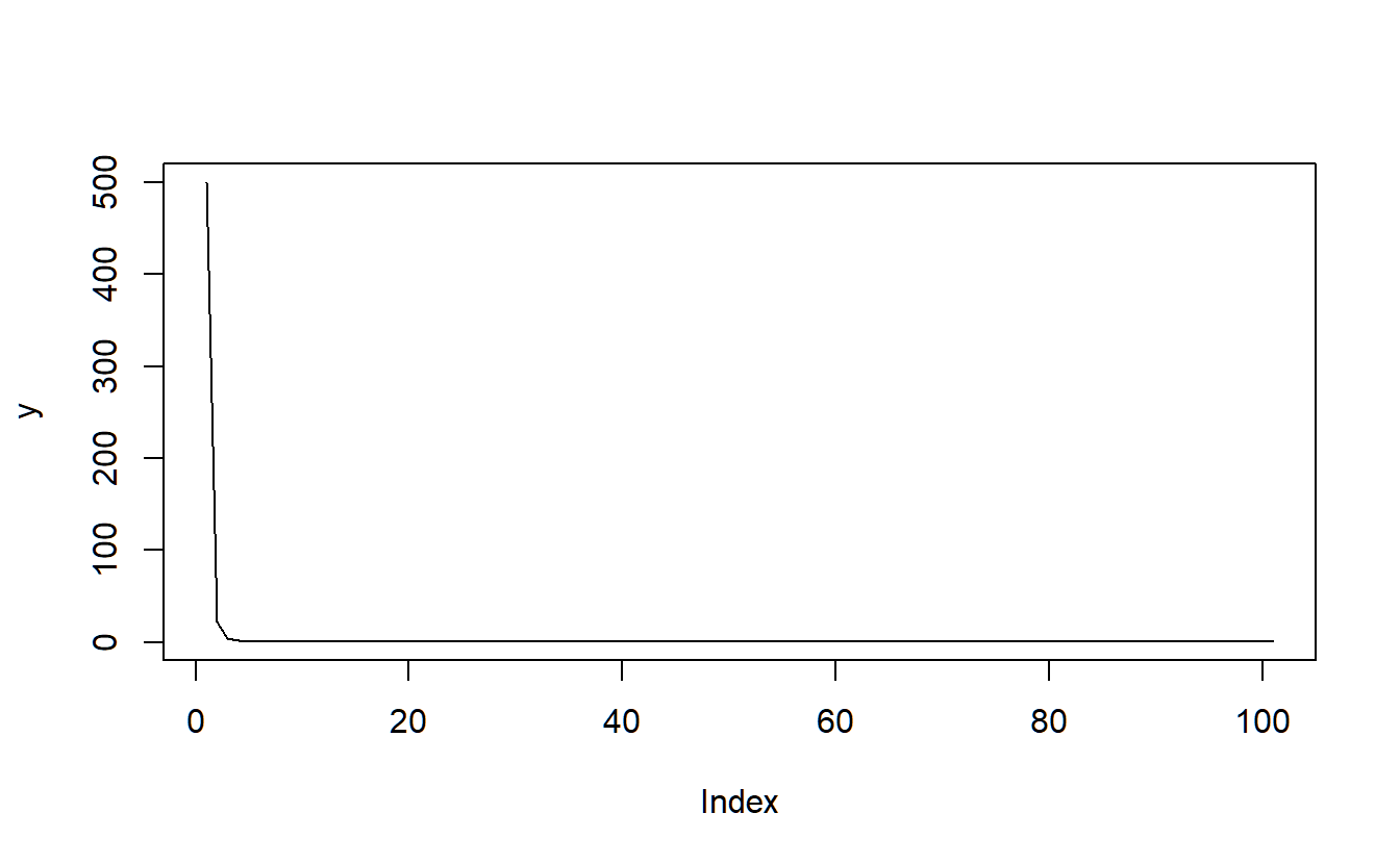
# ASSIGNMENT: lets calculate the 100th square root of the square root of the square root ...
y <- rep(NA,101)
y[1] <- 500
for (i in 1:100){
  if (i%%20==0){print(i)}
  y[i+1] <- sqrt(y[i])
}
#> [1] 20
#> [1] 40
#> [1] 60
#> [1] 80
#> [1] 100
plot(y,type="l")