3 Exploring Data
In this chapter we show how to explore and analyze data using the dataset created in Chapter 2:
discuss frequency and properties of the data (log-returns vs discrete returns)
We load the data and check on it:
#> # A tibble: 2 x 11
#>   symbol company    identifier sedol weight sector    shares_held local_currency
#>   <chr>  <chr>      <chr>      <chr>  <dbl> <chr>           <dbl> <chr>
#> 1 AAPL   Apple Inc. 03783310   2046~ 0.0616 Informat~   168974140 USD
#> 2 MSFT   Microsoft~ 59491810   2588~ 0.0607 Informat~    81130190 USD
#> # ... with 3 more variables: last.sale.price <dbl>, market.cap <dbl>,
#> #   ipo.year <int>
3.1 Plotting and Charting Data
In this chapter we show how to create various graphs of financial time series and their properties, which should help us to get a better understanding of their properties, before we go on to calculate and test their statistics.
3.1.1 Time-series plots
We can now directly plot the return series using a bar-chart. In the following, I
stocks.returns.monthly %>% select(symbol, date, return) %>%
  ggplot(aes(x=date,y=return,col=symbol)) + geom_bar(stat = "identity") + facet_wrap(~symbol)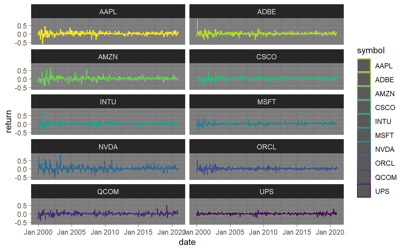
Often we want to relate the performance of different investments in a graphical manner. This can be done by assuming an investment of one dollar at a particular point in time and plotting the resulting cumulated timeseries. We aggregate arithmetic returns as \(R_{1:t}=\prod_{s=0}^{t}(1+R_{s})\). The resulting series is depicted below with the y-scale being log-transformed due to the extraordinary perfromance of sum of the companies in relation to others.
stocks.returns.monthly %>% select(symbol, date, return) %>% mutate(wealth=cumprod(1+return)) %>%
  ggplot(aes(x=date,y=wealth,col=symbol)) + geom_line() + scale_y_log10()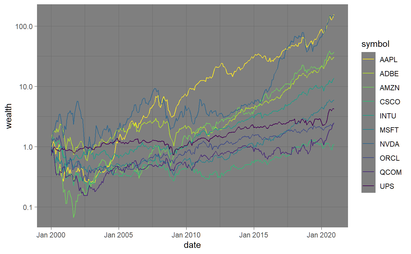
Another series that is rather important when talking about performance is drawdown which describes the decline from a historical peak in a cumulated return series. Unfortunately the function to calculate Drawdowns() per se is only available for xts-input, therefore we stick to only plotting
stocks.returns.monthly %>% select(symbol, date, return) %>% mutate(dd = Drawdowns(return %>% timetk::tx_xts()))
A similar chart can be produced by means of the PerformanceAnalytics package:
stocks.returns.monthly %>% select(symbol, date, return) %>% mutate(wealth=cumprod(1+return)) %>%
  ggplot(aes(x=date,y=wealth,col=symbol)) + geom_line() + scale_y_log10()
3.1.4 Quantile Plots
Putting it all together:
pm <- GGally::ggpairs(iris)
#> Registered S3 method overwritten by 'GGally':
#>   method from
#>   +.gg   ggplot2
if(output %in% c("latex","docx")){
  pm
} else if(output == "html"){
  plotly::ggplotly(pm)
} else(print("No format defined for this output filetype"))
#> `stat_bin()` using `bins = 30`. Pick better value with `binwidth`.
#> `stat_bin()` using `bins = 30`. Pick better value with `binwidth`.
#> Warning: Can only have one: highlight
#> `stat_bin()` using `bins = 30`. Pick better value with `binwidth`.
#> Warning: Can only have one: highlight
#> `stat_bin()` using `bins = 30`. Pick better value with `binwidth`.
#> Warning: Can only have one: highlight
3.2 Analyzing Data
3.2.1 Calculating Statistics and testing and factor exposure
simple and by using performanceanalytics through tidyquant
summary statistics, sample mean and covariance estimation higher moments, tests for (multivariate) normality, quantiles and other risk measures per asset/time period, auto-correlation and predictability?
factor analysis, betas, alphas
3.2.6 Exposure to Factors
The stocks in our example all have a certain exposure to risk factors (e.g. the Fama-French-factors we have added to our dataset). Let us specify these exposures by regression each stocks return on the factors Mkt.RF, SMB and HML using the methods from section 1.2.3