1 Introduction
In the following chapter… [TBD]
1.1 Introduction to Time Series
For a general introduction to R please head to Appendix 8 .
Many of the data sets we will be working with have a (mostly regular) time dimension, and are therefore often called time series. In R there are a variety of classes available to handle data, such as vector(), matrix(), data.frame() or their more modern implementation: tibble(). Adding a time dimension creates a time series from these objects. The most common/flexible package in R that handles time series based on the first three formats are extensible Time Series or xts,1 which we will discuss in the following. Afterwards we will introduce the timetk-package that allows xts() to interplay with tibble() to create the most powerful framework to handle (even very large) time-based data sets (most often encountered in finance).
In the past years the community has worked on different attempts to bring together the powerful group_by() feature from the dplyr package with the abilities of xts(), which is the most powerful and most used time series method in finance to date, due to the available interplay with quantmod and other financial packages. The resulting package creates time-aware tibbles and is called tsibble (part of the tidyverts package collection). Another package to transform easily between both packages is timetk.
A large amount of information regarding tibble() and the finance universe is summarized and updated on the business-science.io-Website at http://www.business-science.io/.
In the next part of this section, we will define a variety of date and time classes, before we introduce the data formats xts(), tibble() and tsibble(). Most of these packages come with some excellent vignettes that I will reference for further reading while solely concentrating on the necessary features for portfolio management - the focus of this book.
1.1.1 Date and Time
There some basic date and time functionalities in base-R2, but mostly we will need additional functions to perform necessary tasks. Available date (time) classes are Date(), POSIXct(), (chron()), yearmon(), yearqtr() and timeDate()3).
1.1.1.1 Basic Date and Time Classes
Initially, we start with the date and time classes included in base R that can all be used as time-index for xts(). We start with the most basic as.Date()
# create variable with date as 'string'
d1 <- "2020-01-18"
# str() checks the structure of the R-object
str(d1)
#>  chr "2020-01-18"
# transform to a date object
d2 <- as.Date(d1)
# check object structure
str(d2)
#>  Date[1:1], format: "2020-01-18"
In the second case, R automatically detects the format of the date object, but if the date format is somewhat more complex, one can specify the format (for all available format definitions, see ?strptime())
# Another date string
d3 <- "4/30-2020"
# transform to date specifying the format
# as.Date(d3) will not work
as.Date(d3, "%m/%d-%Y")
#> [1] "2020-04-30"
If we are working with monthly or quarterly data, yearmon() and yearqtr() will be our friends (both functions are coming from the zoo-package that serves as foundation for the xts-package)
# load the xts library
library(xts)
# transform to year & month object
as.yearmon(d1)
#> [1] "Jan 2020"
as.yearmon(as.Date(d3, "%m/%d-%Y"))
#> [1] "Apr 2020"
# transform to year & quarter
as.yearqtr(d1)
#> [1] "2020 Q1"
as.yearqtr(as.Date(d3, "%m/%d-%Y"))
#> [1] "2020 Q2"
Note, that as.yearmon() shows dates in terms of the current locale of our computer (e.g. Austrian German). We can find out about our locale with Sys.getlocale() and set a different locale with Sys.setlocale()
# set time zone to Austrian German
Sys.setlocale("LC_TIME","German_Austria")
#> [1] "German_Austria.1252"
as.yearmon(d1)
#> [1] "Jän 2020"
# set time zone to English
Sys.setlocale("LC_TIME","English")
#> [1] "English_United States.1252"
as.yearmon(d1)
#> [1] "Jan 2020"
For additional time formats, such as weeks and quarters per year, please check section 1.4.1 the end of this chapter where we introduce the tsibble-package.
When our data also includes information on time, we will either need the POSIXct() (which is the basic package behind all times and dates in R) or the timeDate()-package. The latter one includes excellent abilities to work with financial data as demonstrated below. Note that talking about time also requires to talk about timezones! We start with several examples of the POSIXct()-class:
# converts from time object from character to POSIXct
strptime("2020-01-15 13:55:23.975", "%Y-%m-%d %H:%M:%OS")
#> [1] "2020-01-15 13:55:23 GMT"
as.POSIXct("2019-01-05 14:19:12", format="%Y-%m-%d %H:%M:%S", tz="UTC")
#> [1] "2019-01-05 14:19:12 UTC"
We will mainly use the timeDate-package that provides many useful functions for financial timeseries.
An introduction to timeDate by the Rmetrics group can be found at https://www.rmetrics.org/sites/default/files/2010-02-timeDateObjects.pdf.
# load the timedate library
library(timeDate)
# specify dates and times
Dates <- c("1989-09-28","2001-01-15","2004-08-30")
Times <- c( "23:12:55", "10:34:02", "08:30:00")
# merge to combine dates and times
DatesTimes <- paste(Dates, Times)
# extract date
as.Date(DatesTimes)
#> [1] "1989-09-28" "2001-01-15" "2004-08-30"
# create timedate object
as.timeDate(DatesTimes)
#> GMT
#> [1] [1989-09-28 23:12:55] [2001-01-15 10:34:02] [2004-08-30 08:30:00]
We can see, that timeDate() comes along with timezone information (GMT) that is set to our computer’s locale. timeDate() allows us to specify the timezone of origin (zone) as well as the timezone to transfer data to (FinCenter):
# shift from/to different time zones
timeDate(DatesTimes, zone = "Tokyo", FinCenter = "Zurich")
#> Zurich
#> [1] [1989-09-28 15:12:55] [2001-01-15 02:34:02] [2004-08-30 01:30:00]
timeDate(DatesTimes, zone = "Tokyo", FinCenter = "NewYork")
#> NewYork
#> [1] [1989-09-28 10:12:55] [2001-01-14 20:34:02] [2004-08-29 19:30:00]
timeDate(DatesTimes, zone = "NewYork", FinCenter = "Tokyo")
#> Tokyo
#> [1] [1989-09-29 12:12:55] [2001-01-16 00:34:02] [2004-08-30 21:30:00]
# get a list of all financial centers available in Europe that start with "Vad"
listFinCenter("Europe/Vad*")
#> [1] "Europe/Vaduz"   "Europe/Vatican"
as.Date() as well as the timeDate-package allow us to create time sequences that are necessary to manually create time series. Here we make use of the timeSequence() function to generate monthly dates:
# create time sequence using `seq`
dates1 <- seq(as.Date("2020-01-01"), length=5, by="month")
# show
dates1
#> [1] "2020-01-01" "2020-02-01" "2020-03-01" "2020-04-01" "2020-05-01"
# create time sequence using `timeSequence`
dates2 <- timeSequence(from = "2020-01-01", to = "2020-05-31", by = "month")
# show
dates2
#> GMT
#> [1] [2020-01-01] [2020-02-01] [2020-03-01] [2020-04-01] [2020-05-01]
There are several very useful functions in the timeDate-package to determine first/last days of months/quarters/… which we let speak for themselves:
# subtract seven days
dates1 -7
#> [1] "2019-12-25" "2020-01-25" "2020-02-23" "2020-03-25" "2020-04-24"
# find the first day of each month
timeFirstDayInMonth(dates1 -7)
#> GMT
#> [1] [2019-12-01] [2020-01-01] [2020-02-01] [2020-03-01] [2020-04-01]
# find the first day of each quarter
timeFirstDayInQuarter(dates1)
#> GMT
#> [1] [2020-01-01] [2020-01-01] [2020-01-01] [2020-04-01] [2020-04-01]
# find the last day of each month
timeLastDayInMonth(dates1)
#> GMT
#> [1] [2020-01-31] [2020-02-29] [2020-03-31] [2020-04-30] [2020-05-31]
# find the last day of each quarter
timeLastDayInQuarter(dates1)
#> GMT
#> [1] [2020-03-31] [2020-03-31] [2020-03-31] [2020-06-30] [2020-06-30]
# useful for option expiry, e.g. 3rd Friday of each month
timeNthNdayInMonth("2020-01-01",nday = 5, nth = 3)
#> GMT
#> [1] [2020-01-17]
timeNthNdayInMonth(dates1,nday = 5, nth = 3)
#> GMT
#> [1] [2020-01-17] [2020-02-21] [2020-03-20] [2020-04-17] [2020-05-15]
If we want to create a more specific sequence of times, this can be done with the timeCalendar() function using time ‘atoms’:
# create time sequence using 'atoms'
timeCalendar(m = 1:4, d = c(28, 15, 30, 9), y = c(1989, 2001, 2004, 1990),
             FinCenter = "Europe/Zurich")
#> Europe/Zurich
#> [1] [1989-01-28 01:00:00] [2001-02-15 01:00:00] [2004-03-30 02:00:00]
#> [4] [1990-04-09 02:00:00]
timeCalendar(d=1, m=3:4, y=2020, h = c(9, 14), min = c(15, 23), s=c(39,41),
             FinCenter = "Europe/Zurich", zone = "UTC")
#> Europe/Zurich
#> [1] [2020-03-01 10:15:39] [2020-04-01 16:23:41]
1.1.1.2 Week-days and Business-days
One of the most important functionalities only existing in the timeDate-package is the possibility to check for business days in almost any timezone. The most important ones can be called by holidayXXX()
# holidays at the New York Stock Exchange
holidayNYSE()
#> NewYork
#> [1] [2021-01-01] [2021-01-18] [2021-02-15] [2021-04-02] [2021-05-31]
#> [6] [2021-07-05] [2021-09-06] [2021-11-25] [2021-12-24]
# various holidays in 2021
holiday(year = 2021, Holiday = c("GoodFriday","Easter","FRAllSaints"))
#> GMT
#> [1] [2021-04-02] [2021-04-04] [2021-11-01]
Now we use the Easter holidays of the current year in Europe to first determine weekdays and then business days in Zurich within the 14 days around Easter. To help us along we will use several functions from the lubridate-package.
The lubridate-package is part of the tidyverse collection of R packages for data science. We will introduce the tidyverse in more detail in section 1.2 below.
- Website of the
lubridate-package: https://lubridate.tidyverse.org/ - Corresponding chapter in R for Data Science by Hadley Wickham and Gareth Grolemund: https://r4ds.had.co.nz/dates-and-times.html
- Cheatsheet: https://rawgit.com/rstudio/cheatsheets/master/lubridate.pdf
library(lubridate)
dateSeq <- timeSequence(Easter(year(Sys.time()), -7),
                        Easter(year(Sys.time()), +7))
dayOfWeek(dateSeq)
#> 2021-03-28 2021-03-29 2021-03-30 2021-03-31 2021-04-01 2021-04-02 2021-04-03
#>      "Sun"      "Mon"      "Tue"      "Wed"      "Thu"      "Fri"      "Sat"
#> 2021-04-04 2021-04-05 2021-04-06 2021-04-07 2021-04-08 2021-04-09 2021-04-10
#>      "Sun"      "Mon"      "Tue"      "Wed"      "Thu"      "Fri"      "Sat"
#> 2021-04-11
#>      "Sun"
# select only weekdays
dateSeq2 <- dateSeq[isWeekday(dateSeq)]
dayOfWeek(dateSeq2)
#> 2021-03-29 2021-03-30 2021-03-31 2021-04-01 2021-04-02 2021-04-05 2021-04-06
#>      "Mon"      "Tue"      "Wed"      "Thu"      "Fri"      "Mon"      "Tue"
#> 2021-04-07 2021-04-08 2021-04-09
#>      "Wed"      "Thu"      "Fri"
# select only Business Days in Zurich
dateSeq3 <- dateSeq[isBizday(dateSeq, holidayZURICH(year(Sys.time())))]
dayOfWeek(dateSeq3)
#> 2021-03-29 2021-03-30 2021-03-31 2021-04-01 2021-04-06 2021-04-07 2021-04-08
#>      "Mon"      "Tue"      "Wed"      "Thu"      "Tue"      "Wed"      "Thu"
#> 2021-04-09
#>      "Fri"
Now, one of the strongest points for the timeDate-package is made, when we put times and dates from different time zones together. This could be a challenging task (imagine hourly stock prices from London, Tokyo and New York). Luckily the timeDate-package can handle this easily:
# Series of dates transferred to time zone Zurich/Switzerland
ZH <- timeDate("2021-01-01 16:00:00", zone = "GMT", FinCenter = "Zurich")
# Series of dates transferred to time zone New York/USA
NY <- timeDate("2021-01-01 18:00:00", zone = "GMT", FinCenter = "NewYork")
# Combine both objects
c(ZH, NY)
#> Zurich
#> [1] [2021-01-01 17:00:00] [2021-01-01 19:00:00]
# the Financial Center of the first object is chosen
c(NY, ZH)
#> NewYork
#> [1] [2021-01-01 13:00:00] [2021-01-01 11:00:00]
1.1.2 eXtensible Timeseries
The xts() format is based on the (older) timeseries format zoo(), but extends its power to be more compatible with other data classes. For example, if one converts dates from timeDate, xts() will be so flexible as to memorize the financial center the dates were coming from and upon re-transformation to this class will be reassigned values that would have been lost upon transformation to a pure zoo-object. As quite often we (might) want to transform our data to and from xts this is a great feature and makes our lives a lot easier. Also xts comes with a bundle of other features.
For the reader who wants to dig deeper, we recommend the excellent zoo and xts vignettes:
-
vignette("zoo-quickref"): Quickzoorefernces -
vignette("zoo"): A more general introduction -
vignette("zoo-faq"): FAQ regardingzooobjects -
vignette("zoo-design")andvignette("zoo-read"): Additional information -
vignette("xts"): Very detailedxtsvignette -
vignette("xts-faq"): FAQ forxtsobjects
To start, we load xts and create our first xts() object consisting of a series of randomly created data points:
library(xts)
# set seed to create identical random numbers
set.seed(1)
# create std. normally distributed random numbers
data <- rnorm(3)
# create sequence of dates
dates <- seq(as.Date("2020-05-01"), length=3, by="days")
# form the xts object
xts1 <- xts(x=data, order.by=dates)
# show
xts1
#>              [,1]
#> 2020-05-01 -0.626
#> 2020-05-02  0.184
#> 2020-05-03 -0.836
If one wants to access the data of the time information of this xts object:
# access data
c(zoo::coredata(xts1))
#> [1] -0.626  0.184 -0.836
# access time (index)
zoo::index(xts1)
#> [1] "2020-05-01" "2020-05-02" "2020-05-03"
Here, the xts object was built from a vector and a series of Dates. We could also have used timeDate(), yearmon() or yearqtr() and a data.frame:
# create two data objects (vectors)
s1 <- rnorm(3); s2 <- 1:3
# combine vectors into data.frame
data <- data.frame(s1,s2)
# create time sequence
dates <- timeSequence("2021-01-01",by="months",length.out=3)
# create xts
xts2 <- xts(x=data, order.by=dates)
# show first lines of xts
head(xts2)
#>               s1 s2
#> 2021-01-01  1.60  1
#> 2021-02-01  0.33  2
#> 2021-03-01 -0.82  3
# transform dates to yearmon
dates2 <- as.yearmon(dates)
# create another xts
xts3 <- xts(x=data, order.by = dates2)
# show first lines of xts
head(xts3)
#>             s1 s2
#> Jan 2021  1.60  1
#> Feb 2021  0.33  2
#> Mar 2021 -0.82  3
In the next step we evaluate the merging of two timeseries:
set.seed(1)
# create additional xts
xts3 <- xts(rnorm(3), timeSequence(from = "2020-01-01", to = "2020-03-01", by="month"))
xts4 <- xts(rnorm(3), timeSequence(from = "2020-02-01", to = "2020-04-01", by="month"))
# give names to each time series
colnames(xts3) <- "tsA"; colnames(xts4) <- "tsB"
# merge time series
merge(xts3,xts4)
#>               tsA   tsB
#> 2020-01-01 -0.626    NA
#> 2020-02-01  0.184  1.60
#> 2020-03-01 -0.836  0.33
#> 2020-04-01     NA -0.82
Please be aware that joining timeseries in R does sometimes want you to do a left/right/inner/outer join (aka merge) of the two objects
# left join
merge(xts3,xts4,join = "left")
#>               tsA  tsB
#> 2020-01-01 -0.626   NA
#> 2020-02-01  0.184 1.60
#> 2020-03-01 -0.836 0.33
# right join
merge(xts3,xts4,join = "right")
#>               tsA   tsB
#> 2020-02-01  0.184  1.60
#> 2020-03-01 -0.836  0.33
#> 2020-04-01     NA -0.82
# inner join
merge(xts3,xts4,join = "inner")
#>               tsA  tsB
#> 2020-02-01  0.184 1.60
#> 2020-03-01 -0.836 0.33
# outer join, filling missing elements with 0 rather than NA
merge(xts3,xts4,join="outer",fill=0)
#>               tsA   tsB
#> 2020-01-01 -0.626  0.00
#> 2020-02-01  0.184  1.60
#> 2020-03-01 -0.836  0.33
#> 2020-04-01  0.000 -0.82
In the next step, we subset and replace parts of xts objects
# create another xts object
xts5 <- xts(rnorm(4), timeSequence(from = "2020-11-01",
                                   to = "2021-02-01", by="month"))
# show specific date
xts5["2021-01-01"]
#>             [,1]
#> 2021-01-01 0.576
# show range of dates
xts5["2021-01-01/2021-02-12"]
#>              [,1]
#> 2021-01-01  0.576
#> 2021-02-01 -0.305
# replace element with NA (not available)
xts5[c("2021-01-01")] <- NA
# replace several elements with 99
xts5["2020"] <- 99
# show elemnts starting at
xts5["2020-12-01/"]
#>              [,1]
#> 2020-12-01 99.000
#> 2021-01-01     NA
#> 2021-02-01 -0.305
# show the first two months
xts::first(xts5, "2 months")
#>            [,1]
#> 2020-11-01   99
#> 2020-12-01   99
# show the last element
xts::last(xts5)
#>              [,1]
#> 2021-02-01 -0.305
Then we handle the missing value introduced before. One possibility is just to omit the missing value using na.omit(). Other possibilities would include the last non-missing value na.locf() or linear interpolation with na.approx().
# delete all rows with NA
na.omit(xts5)
#>              [,1]
#> 2020-11-01 99.000
#> 2020-12-01 99.000
#> 2021-02-01 -0.305
# use the last non-missing value
na.locf(xts5)
#>              [,1]
#> 2020-11-01 99.000
#> 2020-12-01 99.000
#> 2021-01-01 99.000
#> 2021-02-01 -0.305
# use the next non-missing value
na.locf(xts5,fromLast = TRUE,na.rm = TRUE)
#>              [,1]
#> 2020-11-01 99.000
#> 2020-12-01 99.000
#> 2021-01-01 -0.305
#> 2021-02-01 -0.305
# linear approximation of missing values
na.approx(xts5,na.rm = FALSE)
#>              [,1]
#> 2020-11-01 99.000
#> 2020-12-01 99.000
#> 2021-01-01 49.347
#> 2021-02-01 -0.305
There are several helper functions to extract information regarding the time and date information of the series. We use these helpers to extract the periodicity, number of months, quarters and years of the series. Then we use to.period()to change periodicity of the data to a larger level creating a so called OHLC (for _O_pen, _H_igh, _L_ow, _C_lose) data set that we often retrieve from financial service data providers (regularizing tick-data to daily observations).
# determine the periodicity of the time series
periodicity(xts5)
#> Monthly periodicity from 2020-11-01 to 2021-02-01
# number of months
nmonths(xts5)
#> [1] 4
# number of quarters
nquarters(xts5)
#> [1] 2
# number of years
nyears(xts5)
#> [1] 2
# change periodicity to quarters and create OHLC data set
to.period(xts5,period="quarters")
#>            xts5.Open xts5.High xts5.Low xts5.Close
#> 2020-12-01    99.000    99.000   99.000     99.000
#> 2021-02-01    -0.305    -0.305   -0.305     -0.305
Many calculations can be done on/with xts objects. This includes standard calculations but extends to several interesting helper functions.
# round squared series
round(xts5^2,2)
#>               [,1]
#> 2020-11-01 9801.00
#> 2020-12-01 9801.00
#> 2021-01-01      NA
#> 2021-02-01    0.09
# to aggregate time series we create a target time object
ep1 <- endpoints(xts5,on="months",k = 2)
# aggregate by summation
period.sum(xts5, INDEX = ep1)
#>            [,1]
#> 2020-12-01  198
#> 2021-02-01   NA
# aggregate with user-specified function
period.apply(xts5, INDEX = ep1, FUN=mean)
#>            [,1]
#> 2020-12-01   99
#> 2021-02-01   NA
# Create lead, lag and diff series and combine
cbind("original"=xts5,"lag"=stats::lag(xts5,k=-1),
      "lead"=stats::lag(xts5,k=1),
      "differences"=diff(xts5))
#>            original    lag lead differences
#> 2020-11-01   99.000 99.000   NA          NA
#> 2020-12-01   99.000     NA   99           0
#> 2021-01-01       NA -0.305   99          NA
#> 2021-02-01   -0.305     NA   NA          NA
Finally, we will show some applications that go beyond xts, for example the use of lapply() to operate on a list() or rollapply() to perform rolling calculations.
# split xts into a yearly list
xts6_yearly <- split(xts5,f="years")
# apply function to each list element
lapply(xts6_yearly,FUN=mean,na.rm=TRUE)
#> [[1]]
#> [1] 99
#>
#> [[2]]
#> [1] -0.305
# with rollapply we can perform rolling window operations such as
# rolling standard deviation (transform to `zoo` before)
zoo::rollapply(as.zoo(xts5), width=3, FUN=sd, na.rm=TRUE)
#>
#> 2020-12-01  0.0
#> 2021-01-01 70.2
Last and least, we plot() the time series object and save it to a ‘.csv’ file using write.zoo(), then open it again using read.zoo() in combination with as.xts(): Note, that xts extends the basic plotting capabilities of base-R and provides additional information as well as a pre-configured time series design.
# create a temporary filename
tmp <- tempfile()
# save xts into the temporary file
write.zoo(xts2,sep=",",file = tmp)
# re-import from temporary file
# this requires us to transform/recognize the time object as `yearmon`
xts8  <- as.xts(read.zoo(tmp, sep=",", FUN2=as.yearmon, header=TRUE))
# plot the times series object
plot(xts8)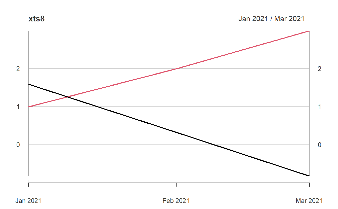
1.2 Introduction to the tidyVerse
Since 2017 a large community effort lead by Hadley Wickham4 went into a collection of open source packages that provide a tidy data approach to import, analyse and model data for data scientists (Wickham et al. 2019). The collection of packages is called the tidyverse and can be simultaneously loaded with library(tidyverse). A tidy data set is a rectangular data matrix that puts variables in columns and observations into rows (Wickham 2014). In contrast to the classical time series representation, where different stocks are represented by columns, dates and/or times are depicted in rows and the elements in the table are prices, returns or market capitalizations.
| Dates | Stock 1 | Stock 2 | … |
|---|---|---|---|
| 2021-01-01 | … | … | … |
| 2021-02-01 | … | … | … |
A tidy version of this data set would have three columns (in long format): Dates, Stock Ids and Returns (plus many more), would be much longer but could also hold more information:
| Dates | Stock Id | Price | Return | … |
|---|---|---|---|---|
| 2021-01-01 | 1 | … | … | |
| 2021-02-01 | 1 | … | … | |
| … | 1 | … | … | |
| 2021-01-01 | 2 | … | … | |
| 2021-02-01 | 2 | … | … |
A representation of such a data set in the tidyverse is called a tibble() and extends the data.frame() by additional requirements on structure and with a much nicer display in the R console. We introduce the tibble() in the next section, together with many convenient commands from dplyr, another package from the tidyverse.
For updates check the tidyverse homepage. A very well written book introducing the tidyverse can be found online: R for Data Science. The core of the tidyverse currently contains several packages:
-
ggplot2for creating powerful graphs (see thevignette("ggplot2-specs")) -
dplyrfor data manipulation (see thevignette("dplyr")) -
tidyrfor tidying data -
readrfor importing datasets (see thevignette("readr")) -
purrrfor programming (see the ``) -
tibblefor modern data.frames (see thevignette("tibble"))
and many more.
1.2.1 Tibbles
We begin this section by loading the tidyverse.
Next, we load the so called FANG data set from the tidyquant package (see chapter 2), containing the daily historical stock prices for the “FANG” tech stocks, “FB” (Facebook), “AMZN” (Amazon), “NFLX” (Netflix), and “GOOG” (Google), spanning from the beginning of 2013 through the end of 2016.
data(FANG, package="tidyquant")The data() command does not produce any output, but loads the data set into the current environment (in RStudio, you would see the name of the data in your Environment tab). To view the data, we can either print the entire data set by typing its name, or we can "slice()" some of the data off to look at just a subset. As of this point we will heavily rely on tools from the tidyverse, such as the pipe-operator %>% that allows us to pipe commands into each other without the necessity of extensively saving intermediary results. For example, in the first line of code below we pipe data using the %>% operator into the slice() function. Essentially, this pipes one command into the other without saving and naming each intermittent step. In a second step, we create a simple tibble(). As mentioned before, a tibble is a ‘tidy’ object with a very concise and clear structure: it has observations in rows and variables in columns. Those variables can have many different formats.
More information on tibbles can be found in (Wickham and Grolemund 2016)’s book R for Data Science: https://r4ds.had.co.nz/tibbles.html
# show the first 5 rows
FANG %>% slice(1:5)
#> # A tibble: 5 x 8
#>   symbol date        open  high   low close   volume adjusted
#>   <chr>  <date>     <dbl> <dbl> <dbl> <dbl>    <dbl>    <dbl>
#> 1 FB     2013-01-02  27.4  28.2  27.4  28   69846400     28
#> 2 FB     2013-01-03  27.9  28.5  27.6  27.8 63140600     27.8
#> 3 FB     2013-01-04  28.0  28.9  27.8  28.8 72715400     28.8
#> 4 FB     2013-01-07  28.7  29.8  28.6  29.4 83781800     29.4
#> 5 FB     2013-01-08  29.5  29.6  28.9  29.1 45871300     29.1
# create an new tibble with three different column formats
tbs1 <- tibble(
  Date = seq(as.Date("2017-01-01"), length=3, by="months"),
  returns = rnorm(3),
  letters = sample(letters, 3, replace = TRUE)
)
# show
tbs1
#> # A tibble: 3 x 3
#>   Date       returns letters
#>   <date>       <dbl> <chr>
#> 1 2017-01-01   1.51  n
#> 2 2017-02-01   0.390 e
#> 3 2017-03-01  -0.621 e
As we can see, all three columns of tbs1 have different formats. One can get the different variables by name and position. To be able to use the pipe operator we often make use the special placeholder operator ..
# extract the returns column as vector
tbs1$returns
#> [1]  1.512  0.390 -0.621
# same with function `pull`
tbs1 %>% pull(returns)
#> [1]  1.512  0.390 -0.621
# get the second column (returns)
tbs1[[2]]
#> [1]  1.512  0.390 -0.621
# similar but using the dot-operator
tbs1 %>% .[[2]]
#> [1]  1.512  0.390 -0.621
Before we analyze a large tibble() such as FANG, we show how to read and save files with tools from the tidyverse. We save the file as ‘csv’ using write_csv() and read it back using read_csv(). Thereby read_csv() guesses (in this case correctly) on the correct column (variable) format.
# vreate temporary file
tmp <- tempfile(fileext = ".csv")
# save tbs1 in file
write_csv(tbs1,file = tmp)
# read back
tbs1b <- read_csv(tmp)
#> Rows: 3 Columns: 3
#> -- Column specification --------------------------------------------------------
#> Delimiter: ","
#> chr  (1): letters
#> dbl  (1): returns
#> date (1): Date
#>
#> i Use `spec()` to retrieve the full column specification for this data.
#> i Specify the column types or set `show_col_types = FALSE` to quiet this message.
# check whether both datasets are similar
dplyr::all_equal(tbs1,tbs1b) # only the factor levels differ
#> [1] TRUE
Another possibility is to save the data-set as an Excel file rather than a ‘csv’ and then read it back into R. We employ the packages readxl and writexl for this task.
While readxl is actually part of the tidyverse it is not automatically loaded and therefore needs library(readxl). In contrast, writexl is not part of the tidyverse, but part of the R open science community that has pledged itself to transform science through open data, software and reproducibility https://ropensci.org/.
# load libraries
library(readxl)
library(writexl)
# temporary file name
tmp <- tempfile(fileext = ".xlsx")
# write to Excel file
writexl::write_xlsx(FANG,path = tmp)
# read from Excel file and transform to date using mutate
FANG3 <- readxl::read_xlsx(tmp) %>% mutate(date=as.Date(date))
# check whether both datasets are similar
dplyr::all_equal(FANG,FANG3)
#> [1] TRUE
Notice that the data looks just the same as when we loaded it from the package. Now that we have the data, we can begin to learn its properties.
# data dimensions
dim(FANG)
#> [1] 4032    8
# names
names(FANG)
#> [1] "symbol"   "date"     "open"     "high"     "low"      "close"    "volume"
#> [8] "adjusted"
# carefully inspect the data
glimpse(FANG)
#> Rows: 4,032
#> Columns: 8
#> $ symbol   <chr> "FB", "FB", "FB", "FB", "FB", "FB", "FB", "FB", "FB", "FB", "~
#> $ date     <date> 2013-01-02, 2013-01-03, 2013-01-04, 2013-01-07, 2013-01-08, ~
#> $ open     <dbl> 27.4, 27.9, 28.0, 28.7, 29.5, 29.7, 30.6, 31.3, 32.1, 30.6, 3~
#> $ high     <dbl> 28.2, 28.5, 28.9, 29.8, 29.6, 30.6, 31.5, 32.0, 32.2, 31.7, 3~
#> $ low      <dbl> 27.4, 27.6, 27.8, 28.6, 28.9, 29.5, 30.3, 31.1, 30.6, 29.9, 2~
#> $ close    <dbl> 28.0, 27.8, 28.8, 29.4, 29.1, 30.6, 31.3, 31.7, 31.0, 30.1, 2~
#> $ volume   <dbl> 6.98e+07, 6.31e+07, 7.27e+07, 8.38e+07, 4.59e+07, 1.05e+08, 9~
#> $ adjusted <dbl> 28.0, 27.8, 28.8, 29.4, 29.1, 30.6, 31.3, 31.7, 31.0, 30.1, 2~
The dim() function tells us that the data has \(4'032\) observations and \(8\) variables. names() lets us check the variable names and glimpse() is designed to give information on the variables as well as give a sample of the data per column.
1.2.2 Summary statistics
Often, we want to know some basics about variables in our data. summary() will give initial statistical information on each variables.
# information on the first three variables
FANG %>% select(symbol,date,open) %>% summary()
#>     symbol               date                 open
#>  Length:4032        Min.   :2013-01-02   Min.   :  23
#>  Class :character   1st Qu.:2014-01-01   1st Qu.: 106
#>  Mode  :character   Median :2015-01-01   Median : 336
#>                     Mean   :2015-01-01   Mean   : 383
#>                     3rd Qu.:2016-01-01   3rd Qu.: 581
#>                     Max.   :2016-12-30   Max.   :1227
The most important commands for tibbles are filter() (filter a variables for certain observations), select() (select variables), arrange() (sort by specified variable), rename() (rename variables) and mutate() (transform variable or create new one). In the following we sort the data set by date, filter for dates after June 2017 and create a new variables return from the adjusted stock prices:
# arrange, filter, rename, mutate, slice
FANG %>%
  arrange(date) %>%
  filter(date>"2016-06-30") %>%
  rename(price=adjusted) %>%
  mutate(return=price/dplyr::lag(price)-1) %>%
  slice(1:5)
#> # A tibble: 5 x 9
#>   symbol date        open  high   low close   volume price return
#>   <chr>  <date>     <dbl> <dbl> <dbl> <dbl>    <dbl> <dbl>  <dbl>
#> 1 FB     2016-07-01  114.  115. 114.  114.  14980000 114.  NA
#> 2 AMZN   2016-07-01  717.  728  717.  726.   2920400 726.   5.36
#> 3 NFLX   2016-07-01   95    97   94.8  96.7 16167200  96.7 -0.867
#> 4 GOOG   2016-07-01  692.  701. 692.  699.   1344700 699.   6.23
#> 5 FB     2016-07-05  114.  114. 113.  114.  14207000 114.  -0.837
Wait! Something is not right. The returns were calculated from one stock to the next one, rather than within stocks. For this to work, we make use of the very important grouping feature of tibble() (dplyr) where group_by() creates groups and calculations are done within groups (here: stocks).
# arrange, filter, mutate
FANG_ret <- FANG %>% group_by(symbol) %>% select(symbol,date,adjusted) %>%
  arrange(date) %>%
  filter(date>"2016-06-30") %>%
  mutate(return=adjusted/dplyr::lag(adjusted)-1)
# show
FANG_ret %>% slice(1:2)
#> # A tibble: 8 x 4
#> # Groups: symbol [4]
#> symbol date adjusted return
#> <chr> <date> <dbl> <dbl>
#> 1 AMZN 2016-07-01 726. NA
#> 2 AMZN 2016-07-05 728. 0.0033
#> 3 FB 2016-07-01 114. NA
#> 4 FB 2016-07-05 114. 0.0001
#> 5 GOOG 2016-07-01 699. NA
#> 6 GOOG 2016-07-05 695. -0.0061
#> # ... with 2 more rowsNow you see, that - despite being arranged by dates - mutate calculates the return within stocks, as expected. Additionally, slice() shows the first two lines per group.
1.2.3 Regression
Mutate() and summarise() can also be used to calculate group-wise regressions. For this we use features of the dplyr-package that were introduced with version 1.0.0 of the package, namely the function nest_by() which combines group_by() and nest() building list-columns that contain all data except the grouping columns. We start by adding an additional column (index) via left_join(), that we calculate as equally weighted average of the four stocks to create an artificial ‘market index.’
FANG_ret2 <- FANG_ret %>% ungroup() %>%
  left_join(FANG_ret %>% group_by(date) %>% summarise(index=mean(return)),by="date") %>%
  select(symbol,date,return,index)
FANG_ret2 %>% group_by(symbol) %>% slice(1:2)
#> # A tibble: 8 x 4
#> # Groups: symbol [4]
#> symbol date return index
#> <chr> <date> <dbl> <dbl>
#> 1 AMZN 2016-07-01 NA NA
#> 2 AMZN 2016-07-05 0.0033 0.0025
#> 3 FB 2016-07-01 NA NA
#> 4 FB 2016-07-05 0.0001 0.0025
#> 5 GOOG 2016-07-01 NA NA
#> 6 GOOG 2016-07-05 -0.0061 0.0025
#> # ... with 2 more rowsNext, we use nest_by() to nest individual stock information into separate tibbles (column data) within the original tibble().
FANG_ret2n <- FANG_ret2 %>% nest_by(symbol)
FANG_ret2n
#> # A tibble: 4 x 2
#> # Rowwise:  symbol
#>   symbol               data
#>   <chr>  <list<tibble[,3]>>
#> 1 AMZN            [127 x 3]
#> 2 FB              [127 x 3]
#> 3 GOOG            [127 x 3]
#> 4 NFLX            [127 x 3]
Next, we calculate a new column model that contains the output of a regression lm() of each stocks return on the index return created above.
FANG_reg <- FANG_ret2n %>%
  mutate(model = list(lm(return ~ index, data = data)))
FANG_reg
#> # A tibble: 4 x 3
#> # Rowwise:  symbol
#>   symbol               data model
#>   <chr>  <list<tibble[,3]>> <list>
#> 1 AMZN            [127 x 3] <lm>
#> 2 FB              [127 x 3] <lm>
#> 3 GOOG            [127 x 3] <lm>
#> 4 NFLX            [127 x 3] <lm>
Finally we can use the functions tidy() and glance() from the broom-package to depict regression output and summary statistics.
#> `summarise()` has grouped output by 'symbol'. You can override using the `.groups` argument.
#> # A tibble: 8 x 6
#> # Groups:   symbol [4]
#>   symbol term        estimate std.error statistic p.value
#>   <chr>  <chr>          <dbl>     <dbl>     <dbl>   <dbl>
#> 1 AMZN   (Intercept)  -0.0004    0.0008    -0.482   0.630
#> 2 AMZN   index         0.810     0.0716    11.3     0
#> 3 FB     (Intercept)  -0.0005    0.0008    -0.672   0.503
#> 4 FB     index         0.727     0.0694    10.5     0
#> 5 GOOG   (Intercept)   0.0003    0.0006     0.428   0.670
#> 6 GOOG   index         0.642     0.0524    12.2     0
#> # ... with 2 more rows
FANG_reg %>%
  summarize(glance(model))
#> `summarise()` has grouped output by 'symbol'. You can override using the `.groups` argument.
#> # A tibble: 4 x 8
#> # Groups: symbol [4]
#> symbol r.squared adj.r.squared sigma statistic p.value df.residual nobs
#> <chr> <dbl> <dbl> <dbl> <dbl> <dbl> <int> <int>
#> 1 AMZN 0.508 0.504 0.009 128. 0 124 126
#> 2 FB 0.470 0.465 0.0088 110. 0 124 126
#> 3 GOOG 0.547 0.543 0.0066 150. 0 124 126
#> 4 NFLX 0.599 0.596 0.0169 185. 0 124 126If we are only interested in the regression coefficients we can modify the initial regression statement to only show regression coefficients (coef()) that we transform into a tibble to preserve the variable names via bind_rows(). The resulting list column then has to be unnest()ed.
FANG_ret2n %>%
  mutate(model = list(bind_rows(coef(lm(return ~ index, data = data))))) %>%
  unnest(model)
#> # A tibble: 4 x 4
#> # Groups: symbol [4]
#> symbol data `(Intercept)` index
#> <chr> <list<tibble[,3]>> <dbl> <dbl>
#> 1 AMZN [127 x 3] -0.00039 0.810
#> 2 FB [127 x 3] -0.00053 0.727
#> 3 GOOG [127 x 3] 0.00025 0.642
#> 4 NFLX [127 x 3] 0.00066 1.82Often in Finance we are also interested in confidence intervals for the regression estimates. In the following we calculate the 5%-confidence interval using confint(), select the one for the first regression coefficient, transform this into a tibble and finally unnest() the resulting list-column.
FANG_reg %>%
  mutate(ci=list(as_tibble(confint(model),rownames="coef"))) %>%
  unnest(ci) %>% select(-data,-model)
#> # A tibble: 8 x 4
#> # Groups: symbol [4]
#> symbol coef `2.5 %` `97.5 %`
#> <chr> <chr> <dbl> <dbl>
#> 1 AMZN (Intercept) -0.002 0.0012
#> 2 AMZN index 0.669 0.952
#> 3 FB (Intercept) -0.0021 0.001
#> 4 FB index 0.59 0.865
#> 5 GOOG (Intercept) -0.0009 0.0014
#> 6 GOOG index 0.538 0.745
#> # ... with 2 more rowsAnother problem occurring frequently in social sciences is the non-normality of the data generating process. Often we observe autocorrelation and heteroskedasticity in the data, that bias our statistics. We can remedy this by using a robust estimator from the sandwich package by means of the coeftest-package.
library(sandwich)
library(lmtest)
FANG_reg %>%
  mutate(lmHC=list(coeftest(model,vcov. = vcovHC(model, type = "HC1")))) %>%
  summarise(broom::tidy(lmHC))
#> `summarise()` has grouped output by 'symbol'. You can override using the `.groups` argument.
#> # A tibble: 8 x 6
#> # Groups: symbol [4]
#> symbol term estimate std.error statistic p.value
#> <chr> <chr> <dbl> <dbl> <dbl> <dbl>
#> 1 AMZN (Intercept) -0.0004 0.0008 -0.495 0.622
#> 2 AMZN index 0.810 0.161 5.04 0
#> 3 FB (Intercept) -0.0005 0.0008 -0.665 0.507
#> 4 FB index 0.727 0.147 4.94 0
#> 5 GOOG (Intercept) 0.0003 0.0006 0.434 0.665
#> 6 GOOG index 0.642 0.0847 7.57 0
#> # ... with 2 more rowsNote, how the statistics associated with the (unchanged) regression estimates vary! More common than the HC1 variance estimate (for more info regarding the various different robust estimators, see ?vcovHC) is the Newey and West (1987) estimator that can be employed using NeweyWest.
FANG_reg %>%
  mutate(lmHC=list(coeftest(model,vcov. = NeweyWest(model))) %>%
  summarise(broom::tidy(lmHC))
#> `summarise()` has grouped output by 'symbol'. You can override using the `.groups` argument.
#> # A tibble: 8 x 6
#> # Groups: symbol [4]
#> symbol term estimate std.error statistic p.value
#> <chr> <chr> <dbl> <dbl> <dbl> <dbl>
#> 1 AMZN (Intercept) -0.0004 0.0007 -0.523 0.602
#> 2 AMZN index 0.810 0.168 4.83 0
#> 3 FB (Intercept) -0.0005 0.0008 -0.693 0.490
#> 4 FB index 0.727 0.143 5.09 0
#> 5 GOOG (Intercept) 0.0003 0.0006 0.444 0.658
#> 6 GOOG index 0.642 0.0915 7.01 0
#> # ... with 2 more rows1.2.4 Plotting
Here we will only give a brief introduction to plotting tidy objects. In 3 we will focus on plotting with regard to the statistical/financial properties of our datasets. In general we use the ggplot2 package to produce simple graphics. ggplot2 has a particular syntax, which looks like this
FANG %>% ggplot(aes(x=date, y=adjusted, color=symbol)) + geom_line()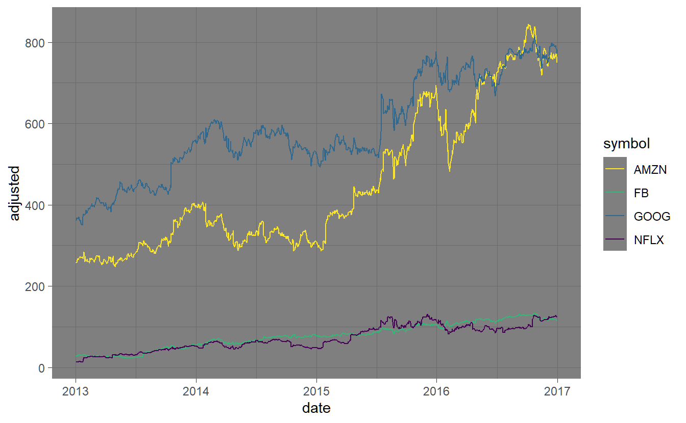
The basic idea is that you need to initialize a plot with ggplot() and then add ‘geoms’ (short for geometric objects) to the plot. The ggplot2 package is based on the Grammar of Graphics, a famous book on data visualization theory. It is a way to map attributes in your data (like variables) to ‘aesthetics’ on the plot. The parameter aes() is short for aesthetic.
For more about the ggplot2 syntax, view the help by typing ?ggplot or ?geom_line. There are also great online resources for ggplot2, like the R graphics cookbook.
To check if our returns have outliers, we can produce boxplots. As usual, a number of options can be specified in order to customize the plots.
FANG_ret %>% ggplot(aes(symbol, return)) + geom_boxplot(aes(color=symbol)) +
  labs(x="symbols", y="returns")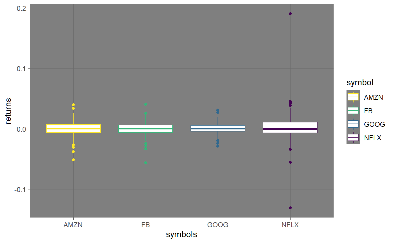
The geom geom_histogram() can be used to plot a histogram including a smooth density using geom_density().
FANG_ret %>% ggplot(aes(return)) +
  geom_histogram(aes(y=..density..)) +
      geom_density(lwd=1) +
facet_wrap(~symbol) + xlab("return") 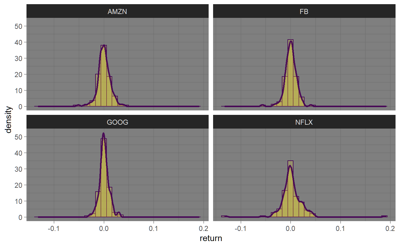
For small data sets, we might want to see all the bivariate relationships between the variables. The GGally package has an extension of the scatterplot matrix that can do just that. We first have to transform our tibble into a wide format (we want relationships between returns for all symbols) using pivot_wider and dismiss the date variable before we pipe the resulting wide tibble into the ggpairs() function. Note that we can save a plot in a variable that we can reuse later (e.g. for saving).
library(GGally)
p <- FANG_ret %>% ungroup() %>% select(date,return, symbol) %>%
  pivot_wider(id_cols = date, names_from = "symbol",
              values_from = "return") %>%
  select(-date) %>% ggpairs()
p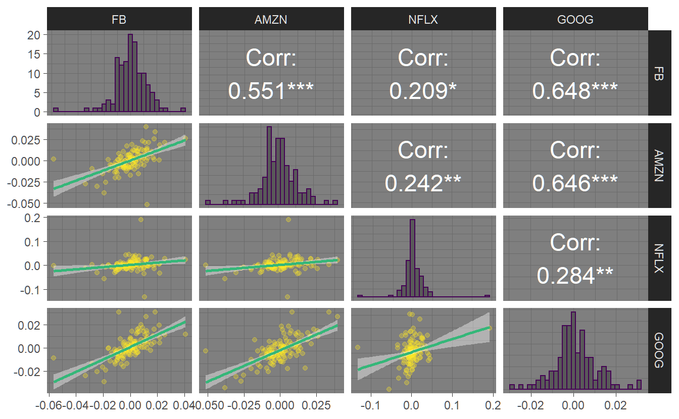
Sometimes, we might want to save a plot for use outside of R. To do this, we can use the ggsave() function, specifying the output format through the filename.
ggsave("ggpairs.png",p1)
1.3 Conversion between tibble and xts
The package timetk was specifically designed to convert between tibble and other (more traditional) timeseries formats like xts or zoo. We will highlight some of its features, again using the (often employed) FANG dataset.
timetk box
To start with, we select only the stock prices of Amazon (symbol AMZN):
library(timetk)
data(FANG)
FANG %>% arrange(symbol) %>% slice(1:2)
#> # A tibble: 2 x 8
#>   symbol date        open  high   low close  volume adjusted
#>   <chr>  <date>     <dbl> <dbl> <dbl> <dbl>   <dbl>    <dbl>
#> 1 AMZN   2013-01-02  256.  258.  253.  257. 3271000     257.
#> 2 AMZN   2013-01-03  257.  261.  256.  258. 2750900     258.
AMZN <- FANG %>% filter(symbol=="AMZN")
One important feature is the possibility to extract the time index (similar to index before),
retrieve more information about the time index via tk_get_timeseries_signature():
tk_index(AMZN) %>% tk_get_timeseries_signature() %>% head(2)
#> # A tibble: 2 x 29
#>   index       index.num  diff  year year.iso  half quarter month month.xts
#>   <date>          <dbl> <dbl> <int>    <int> <int>   <int> <int>     <int>
#> 1 2013-01-02 1357084800    NA  2013     2013     1       1     1         0
#> 2 2013-01-03 1357171200 86400  2013     2013     1       1     1         0
#> # ... with 20 more variables: month.lbl <ord>, day <int>, hour <int>,
#> #   minute <int>, second <int>, hour12 <int>, am.pm <int>, wday <int>,
#> #   wday.xts <int>, wday.lbl <ord>, mday <int>, qday <int>, yday <int>,
#> #   mweek <int>, week <int>, week.iso <int>, week2 <int>, week3 <int>,
#> #   week4 <int>, mday7 <int>
and get some summary information about the time index using tk_get_timeseries_summary():
cat("General summary information\n")
tk_index(AMZN) %>% tk_get_timeseries_summary() %>% head()
#> General summary information
#> # A tibble: 1 x 6
#> n.obs start end units scale tzone
#> <int> <date> <date> <chr> <chr> <chr>
#> 1 1008 2013-01-02 2016-12-30 days day UTC
#> Frequency summary information
#> # A tibble: 1 x 6
#> diff.minimum diff.q1 diff.median diff.mean diff.q3 diff.maximum
#> <dbl> <dbl> <dbl> <dbl> <dbl> <dbl>
#> 1 86400 86400 86400 125096. 86400 345600The most important feature for our purpose however, is the possibility to convert between xts and tibble via tk_xts() and tk_tbl(). To get a multivariate timeseries of adjusted stock prices, we first need to convert from a tidy format to a wide format using pivot_wider(). We select the ‘adjusted’ stock price and drop all other variables.
FANG_wide <- FANG %>% select(date,symbol,adjusted) %>%
  pivot_wider(names_from="symbol",values_from = "adjusted")
FANG_xts <- FANG_wide %>% timetk::tk_xts(silent=TRUE)
FANG_xts %>% head(3)
#>              FB AMZN NFLX GOOG
#> 2013-01-02 28.0  257 13.1  361
#> 2013-01-03 27.8  258 13.8  361
#> 2013-01-04 28.8  259 13.7  369
The other way (converting from xts to tibble) can be done with tk_tbl() and pivot_longer. Note that we have lost some information (OHLC) on the way.
FANG2 <- FANG_xts %>% tk_tbl() %>%
  pivot_longer(cols=2:5, names_to = "symbol", values_to = "adjusted") %>%
  select(symbol,date=index,adjusted) %>% arrange(symbol,date)
#> Warning: `type_convert()` only converts columns of type 'character'.
#> - `df` has no columns of type 'character'
FANG2 %>% slice(1:3)
#> # A tibble: 3 x 3
#>   symbol date       adjusted
#>   <chr>  <date>        <dbl>
#> 1 AMZN   2013-01-02     257.
#> 2 AMZN   2013-01-03     258.
#> 3 AMZN   2013-01-04     259.
timetk has many more interesting features to visualize, wrangle, and feature engineer timeseries data for forecasting and machine learning prediction. In particular those are:
- Plotting timeseries
vignette(TK04_Plotting_Time_Series) - Plotting seasonality and correlation
vignette(TK05_Plotting_Seasonality_and_Correlation) - Automatic anomaly detection
vignette(TK08_Automatic_Anomaly_Detection) - Timeseries machine learning
vignette(TK03_Forecasting_Using_Time_Series_Signature) - Timeseries data wrangling
vignette(TK07_Time_Series_Data_Wrangling) - Automatic frequency detection
vignette(TK06_Automatic_Frequency_And_Trend_Selection) - Automatic anomaly detection, see
vignette(TK08_Automatic_Anomaly_Detection)
1.4 Other useful packages
1.4.1 Tsibble (Time aware tibble)
tsibbles expand tibbles to be aware of their time dimension and comes from the tidyverts package collection.
The tidyverts package collection features several interesting packages build on top of the tsibble:
Be aware, that the team that developed the timetk-package claims that timetk can do all of this within its framework!
We start by creating a tsibble (as_tsibble()) from the dataset used above where we calculated returns for the ‘FANG’ dataset.
library(tsibble)
data(FANG)
FANG_tsbl <- FANG_ret %>%
  select(date,symbol,return) %>%
  as_tsibble(index = date, key=symbol)
FANG_tsbl %>% slice(1:2)
#> # A tsibble: 8 x 3 [1D]
#> # Key:       symbol [4]
#> # Groups:    symbol [4]
#>   date       symbol     return
#>   <date>     <chr>       <dbl>
#> 1 2016-07-01 AMZN   NA
#> 2 2016-07-05 AMZN    0.00333
#> 3 2016-07-01 FB     NA
#> 4 2016-07-05 FB      0.0000875
#> 5 2016-07-01 GOOG   NA
#> 6 2016-07-05 GOOG   -0.00609
#> # ... with 2 more rows
We already know the group_by() feature of the tidyverse. tsibbles add the possibility to do such a group_by() for the time index with index_by(). In this case, we can use it to create monthly moments (mean and standard deviation) without knowing how many days per month there are.
FANG_tsbl %>%
  index_by(year_month = ~ yearmonth(.)) %>% # monthly aggregates
  group_by_key() %>%
  summarise(
    mu = mean(return, na.rm = TRUE),
    sigma = sd(return, na.rm = TRUE)
  ) %>% slice(1:2)
#> # A tsibble: 2 x 4 [1M]
#> # Key:       symbol [1]
#>   symbol year_month       mu   sigma
#>   <chr>       <mth>    <dbl>   <dbl>
#> 1 AMZN     2016 Jul 0.00238  0.00827
#> 2 AMZN     2016 Aug 0.000607 0.00618
Another useful feature is the possibility to fill missing values (dates without observations) by using fill_gaps() (determined using has_gaps(), count_gaps() and scan_gaps()).
FANG_tsbl %>% has_gaps()
#> # A tibble: 4 x 2
#>   symbol .gaps
#>   <chr>  <lgl>
#> 1 AMZN   TRUE
#> 2 FB     TRUE
#> 3 GOOG   TRUE
#> 4 NFLX   TRUE
FANG_tsbl %>%
  fill_gaps(return = 0) %>%
  head(5)
#> # A tsibble: 5 x 3 [1D]
#> # Key:       symbol [1]
#> # Groups:    symbol [1]
#>   date       symbol   return
#>   <date>     <chr>     <dbl>
#> 1 2016-07-01 AMZN   NA
#> 2 2016-07-02 AMZN    0
#> 3 2016-07-03 AMZN    0
#> 4 2016-07-04 AMZN    0
#> 5 2016-07-05 AMZN    0.00333
1.4.2 Slider
Another interesting use case was the possibility to calculate rolling means and standard deviations (e.g. over daily returns within 3 months). This feature has however largely been replaced by the much easier to use slider-package.
To ease our task we define a function that gives us the last date of a month and calculates the mean and the standard deviation.5
library(slider)
monthly_summary <- function(data){
    summarise(data, date=max(date),
              mean=mean(return,na.rm=TRUE),
              sd=sd(return,na.rm=TRUE),.groups = "keep")
}
FANG_ret %>%
  slide_period_dfr(.i = .$date, "month", monthly_summary,
                   .before=3, .complete=TRUE) %>%
  slice(1:2)
#> # A tibble: 8 x 4
#> # Groups:   symbol [4]
#>   symbol date             mean      sd
#>   <chr>  <date>          <dbl>   <dbl>
#> 1 AMZN   2016-10-31  0.00107   0.0111
#> 2 AMZN   2016-11-30 -0.0000290 0.0140
#> 3 FB     2016-10-31  0.00167   0.00893
#> 4 FB     2016-11-30 -0.000453  0.0124
#> 5 GOOG   2016-10-31  0.00141   0.00827
#> 6 GOOG   2016-11-30 -0.000115  0.00998
#> # ... with 2 more rows
Now imagine you want to calculate average returns and standard deviations for a growing window (.before=Inf). In the chunk below we only show the last row of the data pertaining to the full sample average and standard deviation that are also calculated using summarise. Possible applications of this feature will be highlighted in 3.
FANG_ret %>%
  slide_period_dfr(.i = .$date, "month", monthly_summary,
                   .before=Inf, .complete=TRUE) %>%
  slice((n()-1):n())
#> # A tibble: 8 x 4
#> # Groups:   symbol [4]
#>   symbol date           mean      sd
#>   <chr>  <date>        <dbl>   <dbl>
#> 1 AMZN   2016-11-30 0.000408 0.0132
#> 2 AMZN   2016-12-30 0.000342 0.0128
#> 3 FB     2016-11-30 0.000420 0.0122
#> 4 FB     2016-12-30 0.000131 0.0120
#> 5 GOOG   2016-11-30 0.000819 0.0100
#> 6 GOOG   2016-12-30 0.000832 0.00978
#> # ... with 2 more rows
FANG_ret %>% summarise(mean=mean(return,na.rm=TRUE),
                       sd=sd(return,na.rm=TRUE))
#> # A tibble: 4 x 3
#>   symbol     mean      sd
#>   <chr>     <dbl>   <dbl>
#> 1 AMZN   0.000342 0.0128
#> 2 FB     0.000131 0.0120
#> 3 GOOG   0.000832 0.00978
#> 4 NFLX   0.00231  0.0265
This can also be used to calculate rolling regressions. For this specific example we regress on an equally weighted index of all four stocks.6 More specifically we make use of the slide_period() command to calculate the rolling regression over the last three months independent of the number of days within each month.
regression_summary <- function(df){
    reg <- lm(return ~ index, data=df)
    return(tibble("date"=max(df$date),
                  "alpha"=coef(reg)[1],
                  "beta"=coef(reg)[2]))
}
FANG_ret2 %>%
  summarise(model = slide_period(
    .x = cur_data(),
    .i = date,
    .period="month",
    .f = regression_summary,
    .before = 1,
    .complete = FALSE
  )) %>% unnest(model)
#> # A tibble: 6 x 3
#>   date           alpha  beta
#>   <date>         <dbl> <dbl>
#> 1 2016-07-29  7.96e-19  1
#> 2 2016-08-31  4.02e-18  1.00
#> 3 2016-09-30 -1.57e-18  1
#> 4 2016-10-31 -3.48e-18  1.00
#> 5 2016-11-30 -6.61e-19  1.00
#> 6 2016-12-30 -5.35e-19  1
1.5 Assignments
-
Times and Dates: Create a daily time series for 2021:
- Find the subset of first and last days per month/quarter (uniquely)
- Take December 2020 and remove all weekends and holidays in Zurich (Tokyo)
- create a series of five dates & times in New York. Show them for New York, London and Belgrade
-
xts: Create a monthly time series for 2021 using normally distributed random numbers with mean \(0.05\) and standard deviation \(0.1\):
- Add
NAat one point in the time series. Interpolate with values from before and after as well as their mean. - Create a second time series with overlapping (but not the same) normally distributed random numbers with mean \(0.01\) and standard deviation \(0.02\). Name the variables appropriately, then merge together, keeping all the data, replacing missing values with
NAor \(0\). Calculate the correlations between the two time series usingcor(). Try different methods and see what happens. Which one is the correct correlation between the variables?
- Add
-
The
tidyverse: Based on the regression data set ‘FANG_ret’- conduct a t-test for the mean of each return series using
t.test(). - Modify a., by regressing the return of each stock on a constant using
lm(return ~ 1). Calculate a confidence interval around the mean. - Repeat b., but this time use Newey-West autocorrelation and heteroskedasticity-corrected standard errors via
coeftest().
- conduct a t-test for the mean of each return series using