4 Managing Portfolios
In this chapter we show how to explore and analyze mean-variance efficient portfolios using the data set created in Chapter 2. So, we will learn how to optimize portfolios using the full sample of available data. In chapter 5 we will then turn to a more realistic setting and do an out-of-sample analysis on a rolling basis and introduce you to the techniques of backtesting.
The major workhorse of this chapter is the PortfolioAnalytics-package developed by Peterson and Carl (2018). Note that there exists also the fPortfolio-package which seems especially useful for beginners in R - since it is relatively simple in use. Nevertheless, for more complex portfolio optimization tasks, the slightly more complex PortfolioAnalytics-package provides a wider range of tools.
PortfolioAnalytics comes with an excellent introductory vignette vignette("portfolio_vignette") and includes more documents,
- detailing on the use of
ROI-solversvignette("ROI_vignette"), - how to create custom moment functions
vignette("custom_moments_objectives")and - how to introduce CVaR-budgets [
vignette("risk_budget_optimization")](https://cran.r-project.org/web/packages/PortfolioAnalytics/vignettes/risk_budget_optimization.pdf.
4.1 Introduction
Modern portfolio theory suggests how rational investors should optimize their portfolio(s) of risky assets to take full advantage of diversification effects (Markowitz 1952; Rubinstein 2002). Diversification - and therefore the reason to actually optimize portfolios - is possible, because risk as opposed to return is not additive and depends very much on the pairwise co-movements (correlation) between the (risky) assets. The concepts of modern portfolio theory goes back to Markowitz (1952), who considers asset returns as random variables and estimates their expected return \(\mu\) and risk \(\Sigma\) within the available data sample. The most groundbreaking aspect of Markowitz (1952) comes with the finding that the portfolio risk decreases with an increasing amount of assets within the portfolio (Rubinstein 2002).
Performing mean-variance portfolio optimization basically includes three steps (Markowitz 1952):
- Step 1: estimation of the expected return vector \(\mu\) and and variance-covariance matrix \(\Sigma\).
- Step 2: solving for the mean-variance optimal weights, which minimize the portfolio variance for a given return, or maximize return for a given level of risk. This creates a parabola-shaped (actually hyperbolic) minimum-variance frontier in the \(\mu\)-\(\sigma\)-space. Step 2 allows also incorporating certain (optimization) constraints and objectives - outlined in the further course of this section. Depending on the constraints and objectives in Step 2 the shape and the location of the hyperbola changes (we will also come back to this on a later stage in this chapter).
- Step 3: calculation of the most important mean-variance optimal portfolio weights (in particular, the minimum-variance portfolio as well as the tangency portfolio) determined by Step 2.
As stated in Step 2, the two basic portfolio problems are either to minimize the portfolio risk \(w'\Sigma w\) given a target return \(\bar{r}\) (4.1) or maximize the portfolio return \(w'\mu\) given a target level of risk \(\bar{\sigma}\) (4.2) as follows (Markowitz 1952): \[\begin{align} & \underset{w}{\text{min}} & & w'\hat{\Sigma}w \\ & \text{subject to} & & w'\hat{\mu}=\bar{r}, \\ &&& w'\mathbf{1}=1. \tag{4.1} \end{align}\] and \[\begin{align} & \underset{w}{\text{max}} & & w'\hat{\mu}\\ & \text{subject to} & & w'\hat{\Sigma}w=\bar{\sigma}, \\ &&& w'\mathbf{1}=1. \tag{4.2} \end{align}\]
The solutions to these two problems is a hyperbola that depicts the minimum-variance frontier (see also Step 2 above). The given optimal parameterization comes with the assumptions of:
- minimizing the portfolio risk for a given portfolio return, and vice versa (already explained above)
- being invested with 100% of wealth (
full-investmentconstraint)
- being invested with 100% of wealth (
- no short sales restrictions (unlimited short selling is allowed).
However, there is a broad consensus in the literature (Black and Litterman 1992; DeMiguel et al. 2009; DeMiguel, Garlappi, and Uppal 2009) that this setting represents rather a theoretical concept than a real world investment recommendation. At this point it should be noted that based on the Markowitz (1952) approach, it is possible to apply alternative optimization constraints and/or objectives. For instance mutual funds are often not allowed to enter short positions,20 which makes it necessary to bring in a short-sales constraint (long-only). Moreover, in many cases mutual funds are confronted with certain weighting bounds, meaning that they need to invest a minimum fraction of wealth into certain assets or asset groups (box-constraints or group-constraints, e.g. defined by the fund’s investment goals). Another example would be a hedge fund which follows a dollar neutral weighting approach, or applies alternative risk-measures such as the Conditional Value at Risk (CVaR).
All examples mentioned above show that there exist countless combinations of constraints and objectives for optimizing and establishing a mean-variance efficient investment portfolio, all depending on the investor’s specific goals and needs. Besides, the portfolio re-balancing frequency also presents an important criteria in real world applications (and therefore in backtesting as discussed in 5). All in all, we want to highlight that the process of optimizing a portfolio according to ones own constraints and preferences is a rather complex process.
In the following we therefore discuss the implementation of optimization constraints and objectives provided by the portfolioAnalytics-package. The aim is support the reader with an overview to allow him to implement his own mean-variance efficient investment portfolio.
4.2 Tools for Portfolio Management
4.2.1 The Portfolio Object
We start by first creating a portfolio object. The portfolio object is a so-called S3-object, which means, that it has a certain class (portfolio) describing its properties, behavior and relation to other objects. Usually such an object comes with a variety of methods. To create such an object, we reuse our selected stock data set (stocks.selection) with monthly returns in the long format (stocks.returns.monthly), which we have created in Chapter 2:
stocks.returns.monthly %>% slice(1:2)
#> # A tibble: 20 x 10
#> # Groups:   symbol [10]
#>   symbol date      adjusted  return   sp500  Mkt.RF    SMB     HML     RF    Mom
#>   <chr>  <yearmon>    <dbl>   <dbl>   <dbl>   <dbl>  <dbl>   <dbl>  <dbl>  <dbl>
#> 1 AAPL   Jan 2000     0.795 -0.0731 -0.0418 -0.0474 0.0579 -0.0189 0.0041 0.0192
#> 2 AAPL   Feb 2000     0.879  0.105  -0.0201  0.0245 0.215  -0.0981 0.0043 0.182
#> 3 ADBE   Jan 2000    13.7   -0.160  -0.0418 -0.0474 0.0579 -0.0189 0.0041 0.0192
#> 4 ADBE   Feb 2000    25.3    0.852  -0.0201  0.0245 0.215  -0.0981 0.0043 0.182
#> 5 AMZN   Jan 2000    64.6   -0.278  -0.0418 -0.0474 0.0579 -0.0189 0.0041 0.0192
#> 6 AMZN   Feb 2000    68.9    0.0668 -0.0201  0.0245 0.215  -0.0981 0.0043 0.182
#> # ... with 14 more rows
For the PortfolioAnalytics-package we need our data to be in the xts-format (see 1.1.2). At first we pivot_wider() the stocks.returns.monthly dataset into columns of stocks (identified by their symbols) and then convert it to an xts object using tk_xts() from the timetk-package and multiply by \(100\) to get percentage returns.
returns <- stocks.returns.monthly %>%
  select(symbol,date,return) %>%
  pivot_wider(names_from = symbol, values_from = return) %>%
  tk_xts(silent = TRUE) * 100 # portfolio returns in percent
Now, it is time to initialize the portfolio.spec()-object passing along the names of our assets. Additionally, we define category_labels to later allow for the easy inclusion of group-constraints and weight_seq which has only an internal meaning but is currently necessary to avoid problems with the creation of random portfolios. Afterwards we print() the portfolio (S3) object (most S3 objects come with a printing methods that nicely displays some nice information).
To learn more about S3-objects, I recommend the excellently written text “The S3 object system” in Wickham (2019) book Advanced R. Also note, theat below we use {} to pipe the stocks.selection object containing all the information about our assets into the portfolio.spec() object. This is necessary to prevent the pipe-operator %>% from injecting stocks.selection twice (once the entire object using .) and again only one variable of the object using .$symbol. I suggest to
- read up on the pipe-operator using
?magrittr::%>%`, especially the part 'Using the dot for secondary purposes' (which also explains the use of.`). - check out “Programming with
dplyr” usingvignette("programming")to learn about more complex operations.
pspec <- stocks.selection %>%
  {portfolio.spec(assets = .$symbol,
                  category_labels = .$sector,
                  weight_seq = generatesequence(),
                  message=FALSE)}
print(pspec)
#> **************************************************
#> PortfolioAnalytics Portfolio Specification
#> **************************************************
#>
#> Call:
#> portfolio.spec(assets = .$symbol, category_labels = .$sector,
#>     weight_seq = generatesequence(), message = FALSE)
#>
#> Number of assets: 10
#> Asset Names
#>  [1] "AAPL" "MSFT" "AMZN" "NVDA" "ADBE" "CSCO" "ORCL" "INTU" "QCOM" "UPS"
#>
#> Category Labels
#> Information Technology : AAPL MSFT NVDA ADBE CSCO ORCL INTU QCOM
#> Consumer Discretionary : AMZN
#> Industrials : UPS
Checking the structure (str()) of the pspec object,
str(pspec)
#> List of 6
#>  $ assets         : Named num [1:10] 0.1 0.1 0.1 0.1 0.1 0.1 0.1 0.1 0.1 0.1
#>   ..- attr(*, "names")= chr [1:10] "AAPL" "MSFT" "AMZN" "NVDA" ...
#>  $ category_labels:List of 3
#>   ..$ Information Technology: int [1:8] 1 2 4 5 6 7 8 9
#>   ..$ Consumer Discretionary: int 3
#>   ..$ Industrials           : int 10
#>  $ weight_seq     : int [1:10] 1 2 3 4 5 6 7 8 9 10
#>  $ constraints    : list()
#>  $ objectives     : list()
#>  $ call           : language portfolio.spec(assets = stocks.selection$symbol, category_labels = stocks.selection$sector,      weight_seq = 1:l| __truncated__
#>  - attr(*, "class")= chr [1:2] "portfolio.spec" "portfolio"
we find that it (the S3 object) is internally handled as a list and contains several elements: assets which contains the asset names and initial weights that are equally distributed unless otherwise specified (e.g. portfolio.spec(assets=c(0.6,0.4))), category_labels to categorize assets by sector (or geography etc.), weight_seq (sequence of weights for later use by random_portfolios), constraints that we will set soon, objectives and the call that initialized the object. Given all mentioned we will explain how to set optimization and objective constraints.
4.2.2 Constraints
To iterate, constraints define restrictions and boundary conditions on the weights of a portfolio. Constraints are defined by add.constraint()
specifying certain types and arguments for each type, as well as whether the constraint should be enabled or not (enabled=TRUE is the default).
4.2.2.1 Sum of Weights Constraint
Here we define how much of the available budget/wealth can/must be invested by specifying the maximum/minimum sum of portfolio weights.
In the course of this book we want to invest our entire budget and therefore set type="full_investment" which sets the sum of weights to 1. Alternatively, we can set the type="weight_sum" to have minimum/maximum weight_sum equal to 1. In this case it is recommended to set min_sum equal to 0.99 and
max_sum equal to 1.01 vignette("portfolio_vignette"). Further notice that the full_investment specification is part of Markowitz (1952).
pspec <- pspec %>%
  add.constraint(type="full_investment")
print(pspec)
#> **************************************************
#> PortfolioAnalytics Portfolio Specification
#> **************************************************
#>
#> Call:
#> portfolio.spec(assets = .$symbol, category_labels = .$sector,
#>     weight_seq = generatesequence(), message = FALSE)
#>
#> Number of assets: 10
#> Asset Names
#>  [1] "AAPL" "MSFT" "AMZN" "NVDA" "ADBE" "CSCO" "ORCL" "INTU" "QCOM" "UPS"
#>
#> Category Labels
#> Information Technology : AAPL MSFT NVDA ADBE CSCO ORCL INTU QCOM
#> Consumer Discretionary : AMZN
#> Industrials : UPS
#>
#>
#> Constraints
#> Enabled constraint types
#>      - full_investment
Another common constraint is to have the portfolio dollar-neutral type="dollar_neutral"
(or equivalent formulations specified below). Note that the the term dollar neutral implies implies a long-short investment approach, which holds an equal amount of wealth in both long and short positions.
pspec <- pspec %>%
  add.constraint(type="dollar_neutral")
4.2.2.2 Box Constraint
Box constraints specify upper and lower bounds on the asset weights. If we pass min and max as scalars then the same max and min weights
are set per asset. If we pass vectors (that should be of the same length as the number of assets) we can specify position limits on individual stocks.
pspec <- pspec %>%
  add.constraint(type="box", min=0, max=0.4)
print(pspec)
#> **************************************************
#> PortfolioAnalytics Portfolio Specification
#> **************************************************
#>
#> Call:
#> portfolio.spec(assets = .$symbol, category_labels = .$sector,
#>     weight_seq = generatesequence(), message = FALSE)
#>
#> Number of assets: 10
#> Asset Names
#>  [1] "AAPL" "MSFT" "AMZN" "NVDA" "ADBE" "CSCO" "ORCL" "INTU" "QCOM" "UPS"
#>
#> Category Labels
#> Information Technology : AAPL MSFT NVDA ADBE CSCO ORCL INTU QCOM
#> Consumer Discretionary : AMZN
#> Industrials : UPS
#>
#>
#> Constraints
#> Enabled constraint types
#>      - full_investment
#>      - box
Another special type of box constraints are long-only constraints, where we only allow positive weights per asset.
These are set automatically, if no min and max are set or when we use type="long_only"
pspec <- pspec %>%
  add.constraint(portfolio=pspec, type="box") %>%
  add.constraint(portfolio=pspec, type="long_only")
4.2.2.3 Group Constraints
Group constraints allow the user to specify constraints per groups, such as industries, sectors or geography.21 These groups can be randomly defined, below we will set group constraints for the sectors as specified above. The input arguments are the following:
-
groupslist of vectors specifying the groups of the assets, -
group_labelscharacter vector to label the groups (e.g. size, asset class, style, etc.), -
group_minandgroup_maxspecifying minimum and maximum weight per group, -
group_posto specifying the number of non-zero weights per group (optional).
pspec <- pspec %>%
  add.constraint(type="group",
                 # list of vectors specifying the groups of the assets
                 groups=list(pspec$category_labels$`Information Technology`,
                             pspec$category_labels$`Consumer Discretionary`,
                             pspec$category_labels$`Health Care`),
                 group_min=c(0.1, 0.15,0.1),
                 group_max=c(0.85, 0.55,0.4),
                 group_labels=pspec$category_labels)
4.2.2.4 Position Limit Constraint
The position limit constraint allows the user to specify limits on the number of assets with non-zero, long, or short positions. Its arguments are: max_pos which defines the maximum number of assets with non-zero weights and max_pos_long/ max_pos_short that specify the maximum number of
assets with long (i.e. buy) and short (i.e. sell) positions.22
pspec <- pspec %>%
  add.constraint(type="position_limit", max_pos=3) %>%
  add.constraint(type="position_limit", max_pos_long=3, max_pos_short=3)
print(pspec)
#> **************************************************
#> PortfolioAnalytics Portfolio Specification
#> **************************************************
#>
#> Call:
#> portfolio.spec(assets = .$symbol, category_labels = .$sector,
#>     weight_seq = generatesequence(), message = FALSE)
#>
#> Number of assets: 10
#> Asset Names
#>  [1] "AAPL" "MSFT" "AMZN" "NVDA" "ADBE" "CSCO" "ORCL" "INTU" "QCOM" "UPS"
#>
#> Category Labels
#> Information Technology : AAPL MSFT NVDA ADBE CSCO ORCL INTU QCOM
#> Consumer Discretionary : AMZN
#> Industrials : UPS
#>
#>
#> Constraints
#> Enabled constraint types
#>      - full_investment
#>      - box
#>      - position_limit
#>      - position_limit
4.2.2.5 Diversification Constraint
The diversification constraint enables to set a minimum diversification limit by penalizing the optimizer if the deviation is larger
than 5%. Diversification is defined as \(\sum_{i=1}^{N}w_i^2\) for \(N\) assets.23 Its only argument is the diversification target div_target.
pspec <- pspec %>%
  add.constraint(type="diversification", div_target=0.7)
4.2.2.6 Turnover Constraint
The turnover constraint allows to specify a maximum turnover from a set of initial weights that can either be given or are the weights initially specified for the portfolio object. It is also implemented as an optimization penalty if the turnover deviates more than 5% from the turnover_target.24 Note, that this constraint only makes sense for backtesting purposes (see chapter 5).
pspec <- pspec %>%
  add.constraint(type="turnover", turnover_target=0.2)
4.2.2.7 Target Return Constraint
The target return constraint allows the user to target an average return specified by return_target.
pspec <- pspec %>%
  add.constraint(type="return", return_target=0.007)
4.2.2.8 Factor Exposure Constraint
The factor exposure constraint allows the user to set upper and lower bounds on exposures to risk factors. We will use the factor exposures that we have calculated in 3.2.6. The major input is a vector or matrix B and upper/lower bounds for the portfolio factor exposure. If B is a vector (with length equal to the number of assets), lower and upper bounds must be scalars. If B is a matrix, the number of rows must be equal to the number of assets and the number of columns represent the number of factors. In this case, the length of lower and upper bounds must be equal to the number of factors. B should have column names specifying the factors and row names specifying the assets.
B <- stocks.factor_exposure %>% as.data.frame() %>% column_to_rownames("symbol")
pspec <- pspec %>%
  add.constraint(type="factor_exposure",
                 B=B, lower=c(0.8,0,-1), upper=c(1.2,0.8,0))
4.2.2.9 Transaction Cost Constraint
The transaction cost constraint enables the user to specify (proportional) transaction costs.25 Here we will assume the proportional transaction cost ptc to be equal to 1%. Remark that the transaction cost constraint especially comes into play when we run portfolio back tests (see chapter 5).
pspec <- pspec %>%
  add.constraint(type="transaction_cost", ptc=0.01)
4.2.2.10 Leverage Exposure Constraint
The leverage exposure constraint specifies a maximum level of leverage. Below we set leverage to 1.3 to create a 130/30 portfolio. Note that this constraint only makes sense when we allow for the existence of a risk-free asset. The leverage_exposure constraint type is supported for random, DEoptim, pso and GenSA solvers.
pspec <- pspec %>%
  add.constraint(type="leverage_exposure", leverage=1.3)
4.2.2.11 Checking and en-/disabling constraints
Every constraint that is added to the portfolio object gets a number according to the order it was set. If one wants to update (enable/disable) a specific constraints
this can be done by the indexnum argument.
summary(pspec)
#> $category_labels
#> $category_labels$`Information Technology`
#> [1] 1 2 4 5 6 7 8 9
#>
#> $category_labels$`Consumer Discretionary`
#> [1] 3
#>
#> $category_labels$Industrials
#> [1] 10
#>
#>
#> $weight_seq
#>  [1]  1  2  3  4  5  6  7  8  9 10
#>
#> $assets
#> AAPL MSFT AMZN NVDA ADBE CSCO ORCL INTU QCOM  UPS
#>  0.1  0.1  0.1  0.1  0.1  0.1  0.1  0.1  0.1  0.1
#>
#> $enabled_constraints
#> $enabled_constraints[[1]]
#> An object containing 6 nonlinear constraints.
#>
#> $enabled_constraints[[2]]
#> An object containing 5 nonlinear constraints.
#>
#> $enabled_constraints[[3]]
#> An object containing 4 nonlinear constraints.
#>
#> $enabled_constraints[[4]]
#> An object containing 5 nonlinear constraints.
#>
#>
#> $disabled_constraints
#> list()
#>
#> $enabled_objectives
#> list()
#>
#> $disabled_objectives
#> list()
#>
#> attr(,"class")
#> [1] "summary.portfolio"
# To get an overview on the specs, their indexnum and whether they are enabled
consts <- plyr::ldply(pspec$constraints, function(x){c(x$type,x$enabled)})
consts
#>                V1   V2
#> 1 full_investment TRUE
#> 2             box TRUE
#> 3  position_limit TRUE
#> 4  position_limit TRUE
pspec$constraints[[which(consts$V1=="box")]]
#> An object containing 5 nonlinear constraints.
pspec <- add.constraint(pspec, type="box",
                        min=0, max=0.5,
                        indexnum=which(consts$V1=="box"))
pspec$constraints[[which(consts$V1=="box")]]
#> An object containing 5 nonlinear constraints.
# to disable constraints
pspec$constraints[[which(consts$V1=="position_limit")]]
#> add.constraint(portfolio = pspec, type = "position_limit", max_pos = 3)
          # only specify argument if you do enable the constraint
pspec <- add.constraint(pspec, type="position_limit", enable=FALSE,
                        indexnum=which(consts$V1=="position_limit"))
pspec$constraints[[which(consts$V1=="position_limit")]]
#> An object containing 3 nonlinear constraints.
print(pspec)
#> **************************************************
#> PortfolioAnalytics Portfolio Specification
#> **************************************************
#>
#> Call:
#> portfolio.spec(assets = stocks.selection$symbol, category_labels = stocks.selection$sector,
#>     weight_seq = 1:length(stocks.selection$symbol))
#>
#> Number of assets: 10
#> Asset Names
#>  [1] "AAPL" "MSFT" "AMZN" "NVDA" "ADBE" "CSCO" "ORCL" "INTU" "QCOM" "UPS"
#>
#> Category Labels
#> Information Technology : AAPL MSFT NVDA ADBE CSCO ORCL INTU QCOM
#> Consumer Discretionary : AMZN
#> Industrials : UPS
#>
#>
#> Constraints
#> Enabled constraint types
#>      - full_investment
#>      - box
#>      - position_limit
#> - position_limit4.2.3 Objectives
For an “optimal portfolio” there first has to be specified what is optimal in terms of the relevant (business) objective. Such objectives
(target functions) can be added to the portfolio object with add.objective(). With this function, the user can specify the type of objective to add to the portfolio
object. Currently available are ‘return,’ ‘risk,’ ‘risk budget,’ ‘quadratic utility,’ ‘weight concentration,’ ‘turnover’ and ‘minmax.’ Each type of objective has
additional arguments that need to be specified. Several types of objectives can be added and enabled or disabled by specifying the indexnum argument.
4.2.3.1 Portfolio Risk Objective
Here, the user can specify a ‘risk’ function that should be minimized. We start by adding a risk objective to minimize portfolio variance
(minimum variance portfolio). Another example could be the expected tail loss with a confidence level \(0.95\). Whatever function (even user defined ones are possible,
the name must correspond to a function in R), necessary additional arguments to the function have to be passed as a named list to arguments. Examples are:
pspec <- pspec %>%
  add.objective(type='risk',name='var') %>%
  add.objective(type='risk',name='ETL',
                arguments=list(p=0.95),
                enabled=FALSE)
print(pspec)
#> **************************************************
#> PortfolioAnalytics Portfolio Specification
#> **************************************************
#>
#> Call:
#> portfolio.spec(assets = stocks.selection$symbol, category_labels = stocks.selection$sector,
#>     weight_seq = 1:length(stocks.selection$symbol))
#>
#> Number of assets: 10
#> Asset Names
#>  [1] "AAPL" "MSFT" "AMZN" "NVDA" "ADBE" "CSCO" "ORCL" "INTU" "QCOM" "UPS"
#>
#> Category Labels
#> Information Technology : AAPL MSFT NVDA ADBE CSCO ORCL INTU QCOM
#> Consumer Discretionary : AMZN
#> Industrials : UPS
#>
#>
#> Constraints
#> Enabled constraint types
#>      - full_investment
#>      - box
#>      - position_limit
#>      - position_limit
#>
#> Objectives:
#> Enabled objective names
#>      - var
#> Disabled objective names
#>      - ETL
4.2.3.2 Portfolio Return Objective
The ‘return’ objective allows the user to specify a return function to maximize. Here we add a return objective to maximize the portfolio mean return.
pspec <- pspec %>%
  add.objective(type='return', name='mean')
print(pspec)
#> **************************************************
#> PortfolioAnalytics Portfolio Specification
#> **************************************************
#>
#> Call:
#> portfolio.spec(assets = stocks.selection$symbol, category_labels = stocks.selection$sector,
#>     weight_seq = 1:length(stocks.selection$symbol))
#>
#> Number of assets: 10
#> Asset Names
#>  [1] "AAPL" "MSFT" "AMZN" "NVDA" "ADBE" "CSCO" "ORCL" "INTU" "QCOM" "UPS"
#>
#> Category Labels
#> Information Technology : AAPL MSFT NVDA ADBE CSCO ORCL INTU QCOM
#> Consumer Discretionary : AMZN
#> Industrials : UPS
#>
#>
#> Constraints
#> Enabled constraint types
#>      - full_investment
#>      - box
#>      - position_limit
#>      - position_limit
#>
#> Objectives:
#> Enabled objective names
#>      - var
#>      - mean
#> Disabled objective names
#>      - ETL
4.2.3.3 Portfolio Risk Budget Objective
The portfolio ‘risk budget’ objective allows the user to specify constraints to minimize component contribution (i.e. equal risk contribution) or specify upper and lower bounds on percentage risk contribution. Here we specify that no asset can contribute more than 30% to total portfolio risk.
See the risk budget optimization vignette (vignette("risk_budget_optimization")) for more detailed examples of portfolio optimization with risk budgets.
pspec <- pspec %>%
  add.objective(type="risk_budget", name="var",
                max_prisk=0.3) %>%
  add.objective(type="risk_budget", name="ETL",
                arguments=list(p=0.95), max_prisk=0.3,
                enabled=FALSE)
# for an equal risk contribution portfolio, set min_concentration=TRUE
pspec <- pspec %>%
  add.objective(type="risk_budget", name="ETL",
                arguments=list(p=0.95), min_concentration=TRUE,
enabled=FALSE)4.2.4 Solvers
Solvers are the workhorse of our portfolio optimization framework, and there are a variety of them available to us through the portfolioAnalytics-package. We will briefly
introduce the available solvers. Note that these solvers can be specified through optimize_method in the optimize.portfolio() and optimize.portfolio.rebalancing() method.
4.2.4.1 DEOptim
This solver comes from the R-package DEoptim and is a differential evolution algorithm (a global stochastic optimization algorithm) developed by
Ardia et al. (2021) The help on ?DEoptim gives many more references. There is also an explanatory vignette("DEoptimPortfolioOptimization") on large scale portfolio optimization using the portfolioAnalytics-package.
In section 4.3.3 we will give an example of how to use a differential evolution algorithm for portfolio optimization and show how this compares with the exact solution gained using ROI.
[TBD add example and visualization]
4.2.4.2 Random Portfolios
There are three methods to generate random portfolios contained in portfolioAnalytics:26
- The most flexible but also slowest method is ‘sample.’ It can take leverage, box, group, and position limit constraints into account.
- The ‘simplex’ method is useful to generate random portfolios with the full investment and min box constraints (values for min_sum/ max_sum are ignored). Other constraints (_box ma_x, group and position limit constraints will be handled by elimination) which might leave only very few feasible portfolios. Sometimes it will also lead to sub-optimal solutions.
- Using grid search, the ‘grid’ method only satisfies the min and max box constraints.
We highlight this by setting up example portfolios for all three methods. Therefore we specify a portfolio object using portfolio.spec() and set up leverage and box constraints.
# set up simple portfolio with leverage and box constraints
pspec.rpf <- pspec %>%
  add.constraint(type="leverage",min_sum=0.99, max_sum=1.01) %>%
  add.constraint(type="box", min=0, max=1)
Then we create random portfolios using the three methods:
# generate random portfolios using the 3 methods
rpf1 <- pspec.rpf %>%
  random_portfolios(portfolio=., permutations=5000, rp_method='sample')
rpf2 <- pspec.rpf %>%
  random_portfolios(portfolio=., permutations=5000, rp_method='simplex')
rpf3 <- pspec.rpf %>%
  random_portfolios(portfolio=., permutations=5000, rp_method='grid') %>%
  `colnames<-`(colnames(rpf2))
# add all of them together
rpf <- list("sample"=as_tibble(rpf1), "simplex"=as_tibble(rpf2),
            "grid"=as_tibble(rpf3)) %>% bind_rows(.id="Method")
And finally show all feasible portfolios in a \(\mu\)-\(sigma\)-diagram. To do this we have to calculate mean and standard deviation for all simulated portfolios using the returns provided for all ten assets.
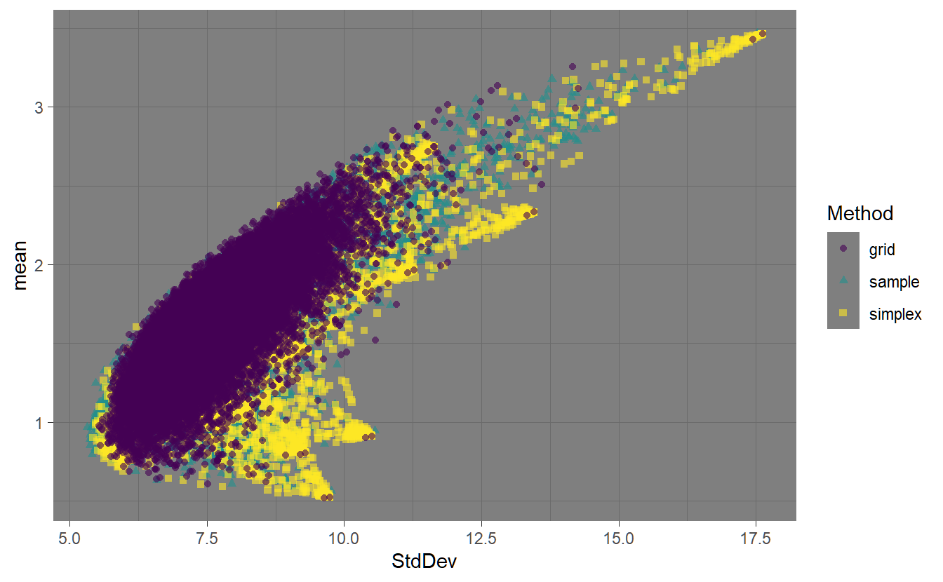
FIGURE 4.1: Highlighting the three different methods for generating random portfolios.
Figure ?? shows the feasible space using the different random portfolio methods. The ‘sample’ method has relatively even coverage of the feasible space. The ‘simplex’ method also has relatively even coverage of the space, but it is also more concentrated around the assets. The ‘grid’ method is pushed to the interior of the space due to the normalization. The fev argument controls the face-edge-vertex biasing. Higher values for fev will result in the weights vector more concentrated on a single asset. This can be seen in the following chart.
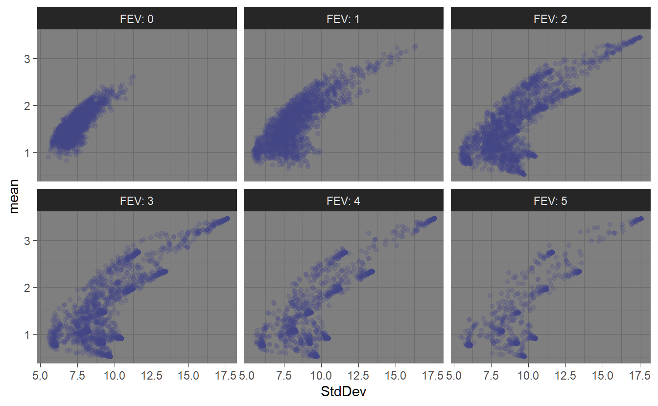
FIGURE 4.2: Effects of the ‘fev’ parameter on random porfolio generation.
In section @(sss-4Optimizer) we will give an example of how to use random portfolios in portfolio optimization and show how they compare with the exact solution gained using ROI.
4.2.4.3 pso
The psoptim function from the R package pso (Bendtsen. 2012) uses particle swarm optimization. [TBD add example and visualization]
In section 4.3.3 we will give an example of how to use particle swarm optimization and show how this compares with the exact solution gained using ROI.
4.2.4.4 GenSA
The GenSA function from the R package GenSA (Gubian et al. 2018) is based on generalized simulated annealing (a generic probabilistic heuristic optimization algorithm). [TBD add example and visualization]
In section 4.3.3 we will give an example of how to use generalized simulated annealing for portfolio optimization and show how this compares with the exact solution gained using ROI.
4.2.4.5 ROI
The ROI (R Optimization Infrastructure) is a framework to handle optimization problems in R. It serves as an interface to the Rglpk package and the quadprog package which solve linear and quadratic programming problems. Available methods in the context of the portfolioAnalytics-package are given below (see section ?? for available objectives.
- Maximize portfolio return subject to leverage, box, group, position limit, target mean return, and/or factor exposure constraints on weights.
- Globally minimize portfolio variance subject to leverage, box, group, turnover, and/or factor exposure constraints.
- Minimize portfolio variance subject to leverage, box, group, and/or factor exposure constraints given a desired portfolio return.
- Maximize quadratic utility subject to leverage, box, group, target mean return, turnover, and/or factor exposure constraints and risk aversion parameter.
(The risk aversion parameter is passed into
optimize.portfolio()as an added argument to the portfolio object). - Minimize ETL subject to leverage, box, group, position limit, target mean return, and/or factor exposure constraints and target portfolio return.
4.2.4.6 Multicore capabilities
For large sets of assets and solvers that can be parallelized, the doParallel-package (Corporation and Weston 2020) provides multi-core capabilities to the portfolioAnalytics package. Therefore we load the doParallel library and initiate a multi-core application using registerDoParallel(). Note, that this automatically detects the number of available cores and uses all of them. Use detectCores() to find out how many CPU-cores you have and use registerDoParallel(cores = 3) to use a different number of cores.
4.2.5 Portfolio Information and Visualization
To highlight everything mentioned above and analyse the results appropriately we finally outline useful visualization commands. In this context the main focus is on the efficient frontier and the corresponding optimal portfolio weights as well as the risk/reward information.
The following visualization commands are available:
-
chart.EfficientFrontier(): Charts the efficient frontier and adds the assets. -
chart.EfficientFrontierOverlay(): Charts various efficient frontiers in the risk-return space. -
chart.EF.Weights(): Chart weights along the efficient frontier. -
chart.Weights(): Chart weights per asset. -
chart.GroupWeights(): Chart weights per group/category. -
chart.RiskBudget(): Plots the (percent) contribution of assets to the objective risk measure. -
chart.RiskReward(): Charts the optimized portfolio object in the risk-return space. -
chart.Concentration(): Charts the optimized portfolio object in risk-return space and adds the degree of concentration based on the component contribution to risk.
4.3 Mean-Variance Optimal Portfolios - Examples
As already outlined, the efficient frontier is hyperbolic shaped and the envelope of all individual/sub-portfolio minimum-variance frontiers. Portfolios located on the dominating (most northwestern) minimum-variance frontier are called efficient. Thus, for given expected return the risk is minimized, or vice versa, for a given risk the return is maximized. Hence, the efficient frontier draws all combinations of portfolio weights which provide the lowest risk for a given return. This could be either interpreted as the minimum risk portfolio for a given return \(\mu\) or the maximum return for a given risk \(\sigma\) (Step 1 and Step 2). Depending on the restrictions or boundary conditions of Step 2 the shape of the hyperbola changes. As a rule of thumb: the fewer restrictions the more efficient (north-westerly) the frontier.
In the course of this example efficient frontiers with different restrictions are analysed:
- Efficient frontiers according to Markowitz (1952).
- Efficient frontiers with a long-only constraint.
- Box-constraint portfolios related to the long-only setting.
- Group-constraint portfolios related to the long-only setting.
4.3.1 Portfolio specifications and the efficient frontier
We have previously shown the different possibilities for mean-variance optimization by introducing different (i) constraints, (ii) objectives and (iii) solvers. Now we will combine all these aspects and highlight the theoretical as well practical results arising from optimization constraints and objectives. As already outlined before, the Markowitz (1952) approach assumes an investor who is being invested with 100% of wealth (full-investment) and not confronted with any short-sale restrictions. Thereon, introducing further optimization constraints results in a less efficient frontier (positioned to the south-east). In order to take a closer look on this fact we first implement the pspec.basic object which defines the assets element of the S3 object, as well as the (basic) full investment constraint.
4.3.1.1 Basic investment example
#> **************************************************
#> PortfolioAnalytics Portfolio Specification
#> **************************************************
#>
#> Call:
#> portfolio.spec(assets = .$symbol, category_labels = .$sector,
#>     weight_seq = generatesequence(), message = FALSE)
#>
#> Number of assets: 10
#> Asset Names
#>  [1] "AAPL" "MSFT" "AMZN" "NVDA" "ADBE" "CSCO" "ORCL" "INTU" "QCOM" "UPS"
#>
#> Category Labels
#> Information Technology : AAPL MSFT NVDA ADBE CSCO ORCL INTU QCOM
#> Consumer Discretionary : AMZN
#> Industrials : UPS
# Set base portfolio spec
pspec.basic <- pspec %>%
  # Set full investment constraint - invest 100% of available wealth
  add.constraint(type = "full_investment")
Thereon we define the Markowitz (1952) pspec.M object by adding both risk and return objectives. Again note, that this portfolio specification allocates
100% of wealth into the 10 available assets without cash position and no short sales restrictions. We can plot the efficient frontier using chart.EfficientFrontier(). We additionally plot the Capital Allocation Line with tangent.line = TRUE which needs to specify the risk-free rate using rf. The number of portfolios to chart along the EF is set via n.portfolios = 100. We also chart and label all the assets using chart.assets = TRUE and labels.assets = TRUE.
# Add objectives
pspec.M <- pspec.basic %>%
  add.objective(type = "return", name = "mean") %>%
  add.objective(type = "risk", name = "StdDev")
# Calculate efficient frontier (with ROI solver)
markowitz.ROI <- optimize.portfolio(returns, pspec.M,
                                    optimize_method = "ROI", trace = TRUE)
# Generate tailored Frontier Plot
chart.EfficientFrontier(markowitz.ROI, match.col = "StdDev",
                        n.portfolios = 100,
                        tangent.line = TRUE, rf=1/12,
                        chart.assets = TRUE, labels.assets = TRUE)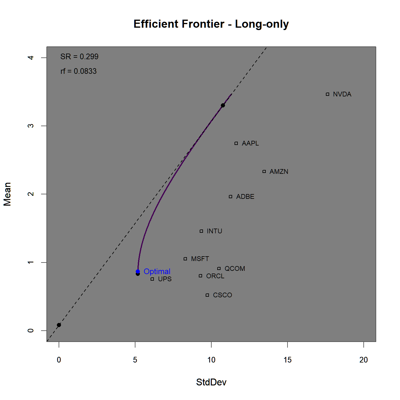
FIGURE 4.3: Efficient frontier and optimal portfolios for the standard Markwoitz (1952) portfolio.
The efficient frontier plot in figure 4.3 consists of \(100\) mean-variance efficient portfolios. Note, how far above (to the north-east) the assets with the highest Sharpe-Ratios are surpassed by the efficient frontier without constraints. This is mainly due to the possibility of short-selling individual assets. To get a better understanding of this, we plot the weights along the efficient frontier (with a reduced number of portfolios n.portfolios = 30).
# Generate plot of weights along the efficient frontier
chart.EF.Weights(markowitz.ROI, n.portfolios = 30, type="mean-StdDev",
                 match.col = "StdDev")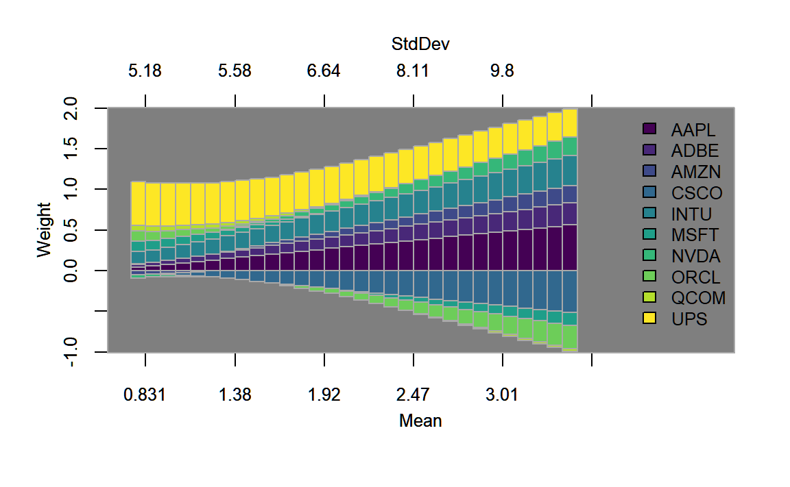
FIGURE 4.4: Weights plotted along the efficient frontier for the standard Markwoitz (1952) portfolio.
In figure 4.4, we find that along the efficient frontier, short selling involves primarily the assets with the lowest return/risk-profile, namely ‘Cisco,’ ‘Microsoft’ and ‘Oracle.’ Other assets that have a low return-risk profile (such as UPS that dominates some of the aforementioned assets) are always in the portfolio, potentially due to their diversification potential. In 4.5 we find evidence to this effect, as ‘UPS’ seems to have the lowest corrrelation with all other assets.
library(GGally)
p <- stocks.returns.monthly %>% ungroup() %>% select(date,return, symbol) %>%
  pivot_wider(id_cols = date, names_from = "symbol",
              values_from = "return") %>%
  select(-date) %>% ggpairs()
p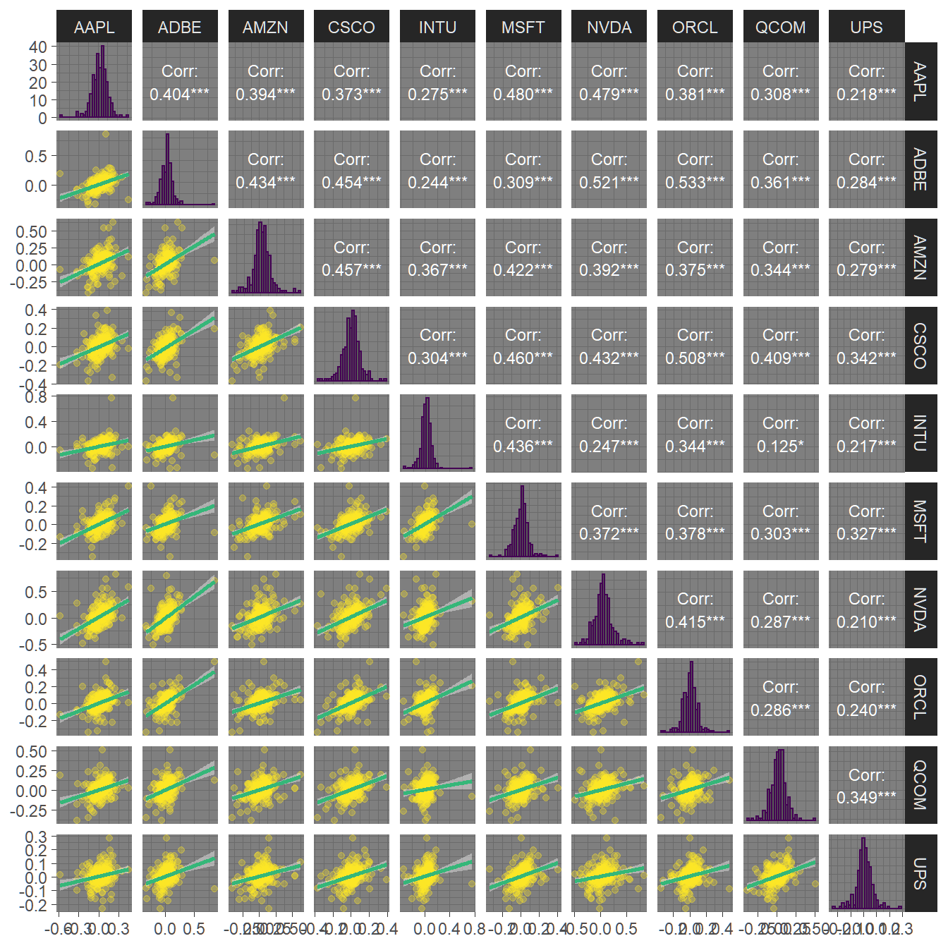
FIGURE 4.5: Pairwise correlations and dependency plots of all ten assets.
These portfolio weights can be saved using the create.EfficientFrontier() function, where we again save all \(100\) portfolio weights.
4.3.1.2 Long-only investment example
In a next step, we impose a long-only constraint by generating the pspec.lo object.
# Only allow long positions
pspec.lo <- pspec.basic %>%
  add.constraint(type = "long_only") %>%
  # Add objectives
  add.objective(type = "return", name = "mean") %>%
  add.objective(type = "risk", name = "StdDev")
# Calculate efficient frontier (with ROI solver)
longonly.ROI <- optimize.portfolio(returns, pspec.lo,
                                   optimize_method = "ROI", trace = TRUE)
chart.EfficientFrontier(longonly.ROI, match.col = "StdDev",
                        n.portfolios = 100,
                        tangent.line = TRUE, rf=1/12,
                        chart.assets = TRUE, labels.assets = TRUE)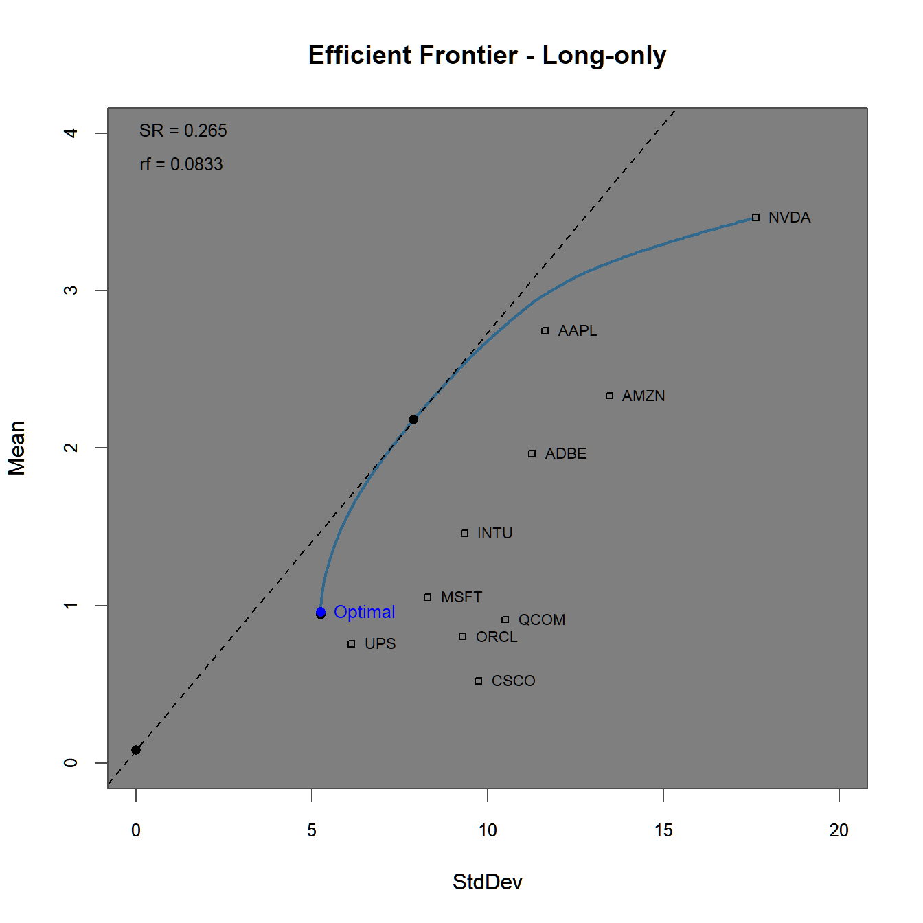
FIGURE 4.6: Efficient frontier and optimal portfolios for the using a long-only constraint.
The efficient frontier plot in figure 4.6 lies below the one generated before in figure 4.3 due to the (implicitely) imposed short-sale constraints. This can additionally be seen in figure 4.7, where the last portfolio fully invests into the asset with the highest individual Sharpe-ratio.
# Generate plot of weights along the efficient frontier
chart.EF.Weights(longonly.ROI, n.portfolios = 30,
                 type="mean-StdDev", match.col = "StdDev")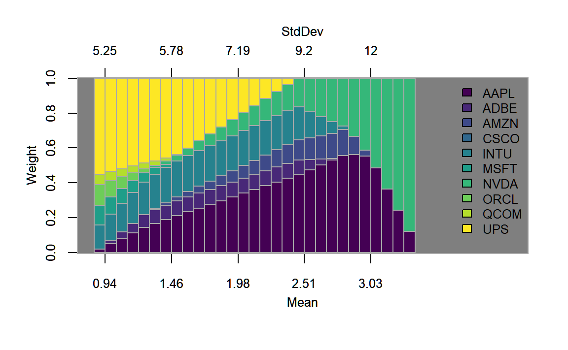
FIGURE 4.7: Weights plotted along the efficient frontier for the portfolio with the long-only constraint.
4.3.1.3 Box-constrained investment example
Next, we add a box constraint to pspec.lo. As outlined at the beginning of this chapter, investment funds are commonly restricted to weight certain assets at a
maximum and/or minimum (upper and lower bounds) levels. The applied box constraint restricts the weight allocation to a minimum of \(5%\) and a maximum of \(40%\).
# Box Constraint
pspec.lo.box <- pspec.lo %>%
  add.constraint(type = "box", name ="x", min=0.05, max=0.4)
  # Calculate efficient frontier
lo.box.ROI <- optimize.portfolio(returns, pspec.lo.box,
                                 optimize_method = "ROI", trace = TRUE)
chart.EfficientFrontier(lo.box.ROI, match.col = "StdDev",
                        n.portfolios = 100,
                        tangent.line = TRUE, rf=1/12,
                        chart.assets = TRUE, labels.assets = TRUE)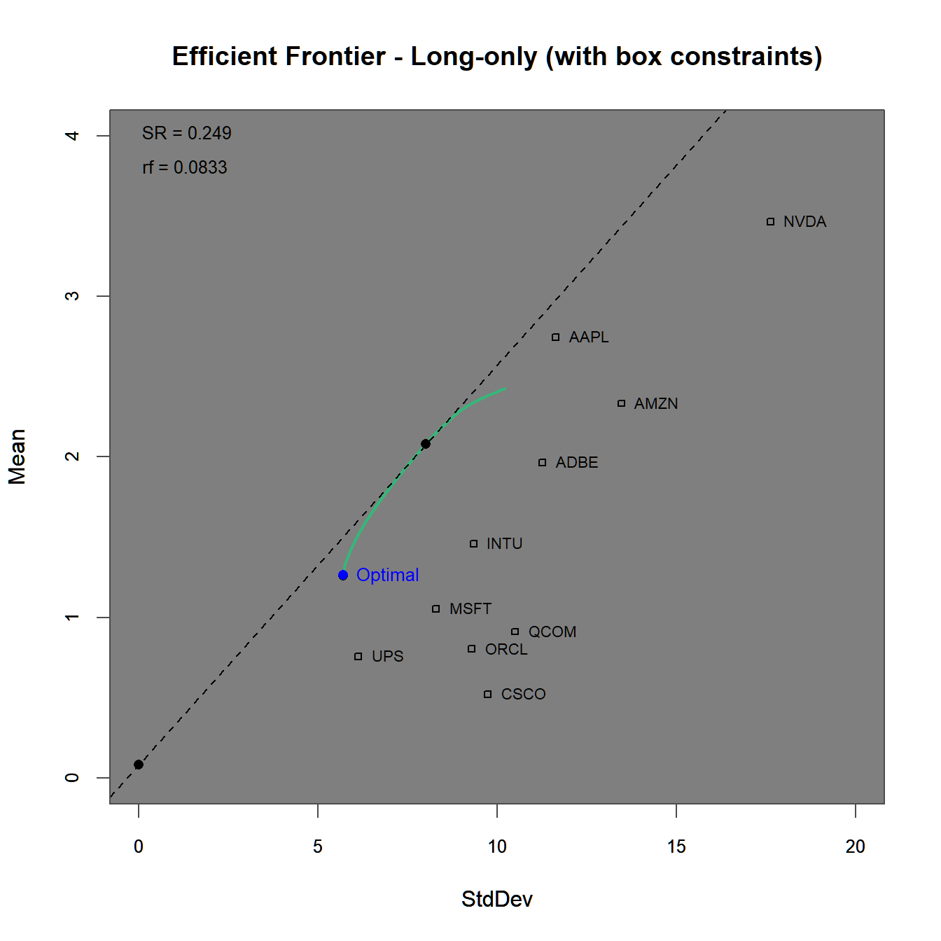
FIGURE 4.8: Efficient frontier and optimal portfolios for the using a long-only as well as a box constraint.
The efficient frontier plot in figure 4.8 lies even further below the one generated before in figures 4.3 and 4.6 due to the stricter constraints. Note, that the efficient frontier does not reach as far as ‘Nvidia’ or ‘Apple’ due to the maximum possible weight of \(40%\), with additional support found in figure 4.8.
# Generate plot of weights along the efficient frontier
chart.EF.Weights(lo.box.ROI, n.portfolios = 30,
                 type="mean-StdDev", match.col = "StdDev")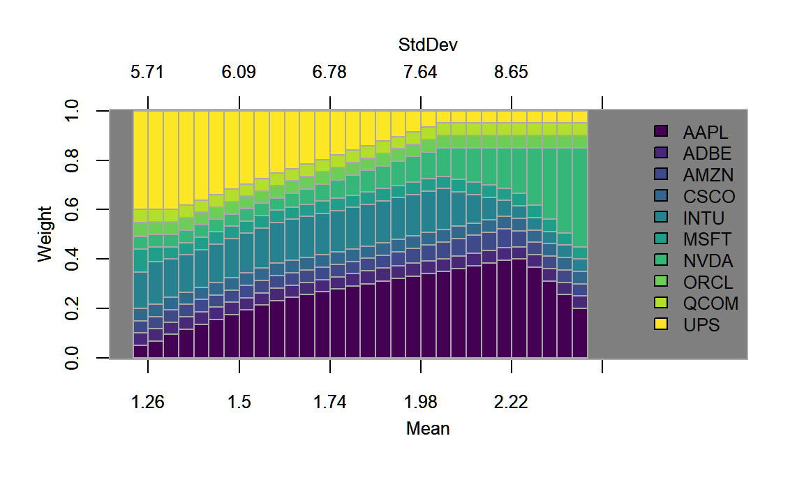
FIGURE 4.9: Weights plotted along the efficient frontier for the portfolio with a long-only as well as a box constraint.
4.3.1.4 Group-constrained investment example
Finally, we add a group constraint to pspec.lo.box to highlight the effect of even further restricting the investment space.
# Box Constraint
pspec.lo.group <- pspec.lo.box %>%
  add.constraint(type="group",
                 # list of vectors specifying the groups of the assets
                 groups=list(pspec$category_labels$`Information Technology`,
                             pspec$category_labels$`Consumer Discretionary`,
                             pspec$category_labels$`Industrials`),
                 group_min=c(0.1, 0.15,0.1),
                 group_max=c(0.4, 0.55,0.4),
                 group_labels=pspec$category_labels)
  # Calculate efficient frontier
lo.group.ROI <- optimize.portfolio(returns, pspec.lo.group,
                                   optimize_method = "ROI", trace = TRUE)
chart.EfficientFrontier(lo.group.ROI, match.col = "StdDev",
                        n.portfolios = 100,
                        tangent.line = TRUE, rf=1/12,
                        chart.assets = TRUE, labels.assets = TRUE)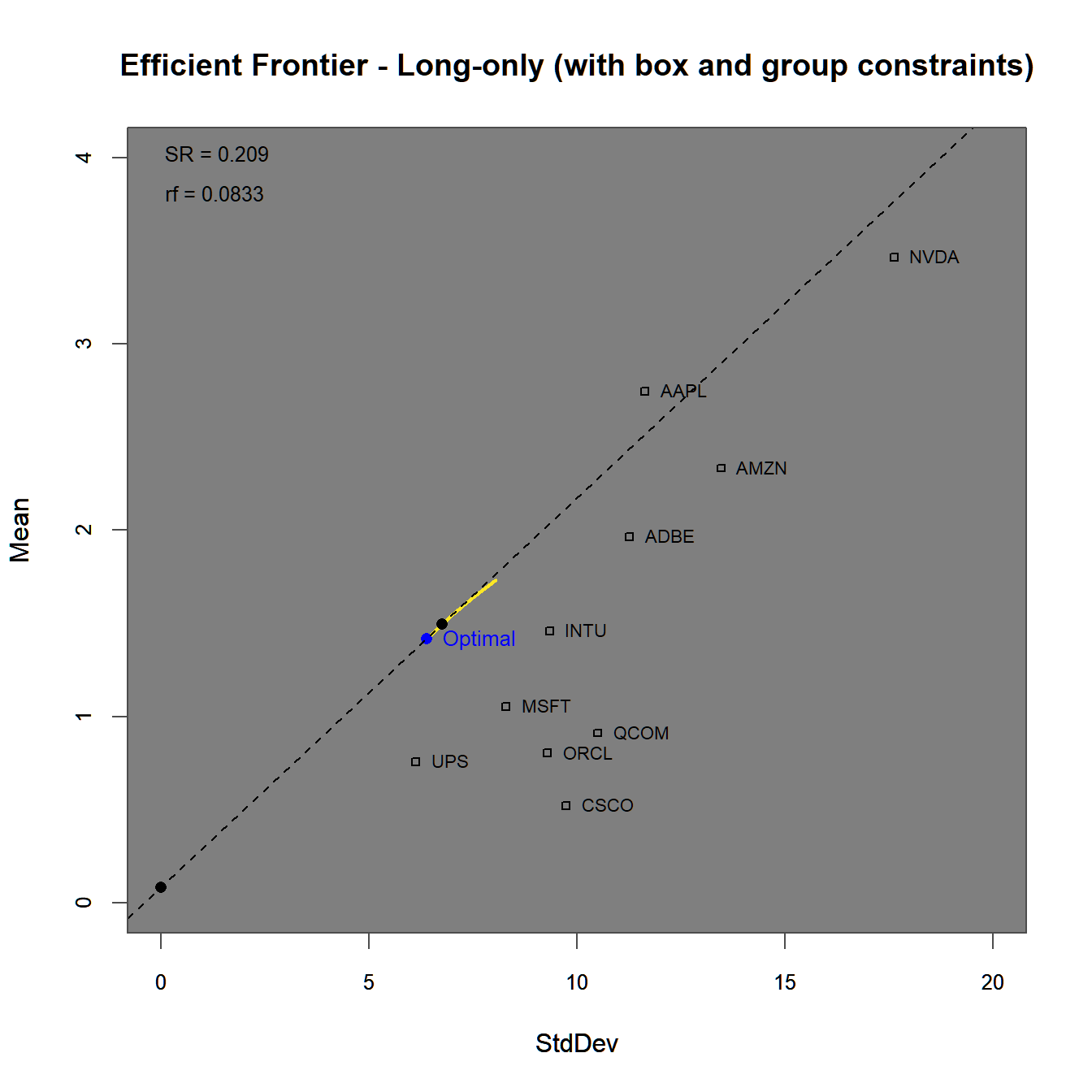
FIGURE 4.10: Efficient frontier and optimal portfolios for the using a long-only as well as a box and a group constraint.
The efficient frontier plot in figure 4.10 lies even further below the one generated above in figure 4.8. Due to the (for demonstration purposes) very tight group constraints, we invest a large portion of our money into ‘UPS’ and ‘Amazon.’
# Generate plot of weights along the efficient frontier
chart.EF.Weights(lo.group.ROI, n.portfolios = 30,
                 type="mean-StdDev", match.col = "StdDev")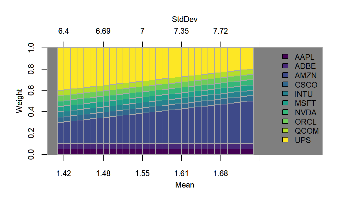
FIGURE 4.11: Weights plotted along the efficient frontier for the portfolio with a long-only as well as a box and a group constraint.
In figure 4.12 we additionally show the weights per group in the optimal portfolio. We find, that within the three groups:
- Information Technology (weight \(\in [0.1,0.4]\)): AAPL MSFT NVDA ADBE CSCO ORCL INTU QCOM
- Consumer Discretionary (weight \(\in [0.15,0.55]\)): AMZN
- Industrials (weight \(\in [0.1,0.4]\)): UPS
only the first and the last group are maximized in terms of the group constraints. Whereas this is natural for the first group to the binding box constraint, that forces these assets to a minimum weight of \(5%\) (which times \(8\) assets equals exactly \(40%\)), the only two assets that could be balanced within these bounds are Amazon \(20%\) and UPS \(40%\).
# Generate plot of group weights for the optimal portfolio
chart.GroupWeights(lo.group.ROI,grouping = c("category"),
                   plot.type="barplot",
                   main="Group-weights")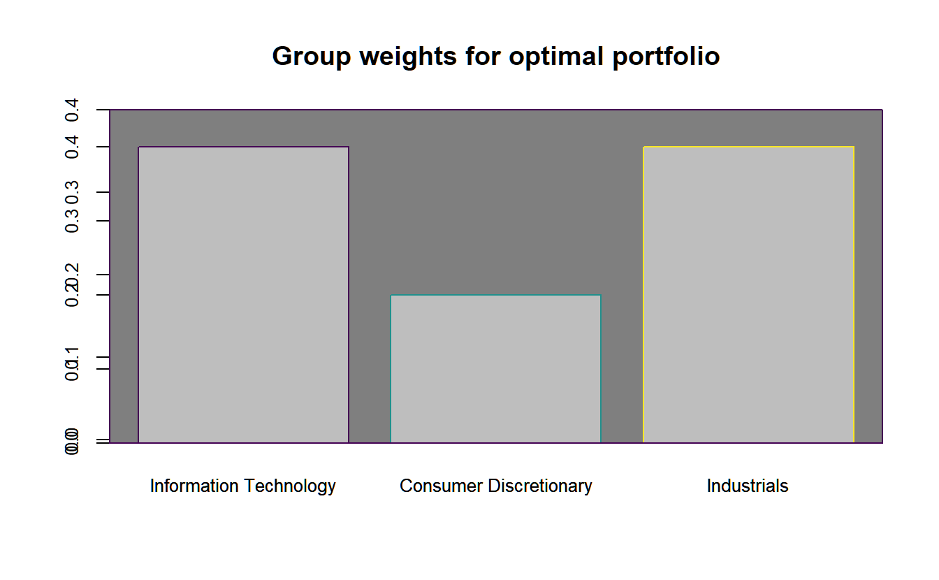
FIGURE 4.12: Weights plotted along the efficient frontier for the portfolio with a long-only as well as a box and a group constraint.
4.3.1.5 Combining the examples
Next we overlay the already calculated portfolio objects pspec.M, pspec.lo, pspec.lo.box using chart.EfficientFrontierOverlay(). For this we first need to create a list comprising the portfolio objects via combine.portfolios().
# Create portfolio object list
portf.list <- list(pspec.M, pspec.lo, pspec.lo.box, pspec.lo.group) %>%
  combine.portfolios()
# Legend of portfolio objects
legend.labels <- c("Markowitz", "Long-Only",
                   "Box-Constraint","Group/Box-Constraint")
chart.EfficientFrontierOverlay(returns, portf.list,
                               type="mean-StdDev", match.col = "StdDev",
                               labels.assets = TRUE,
                               legend.labels = legend.labels)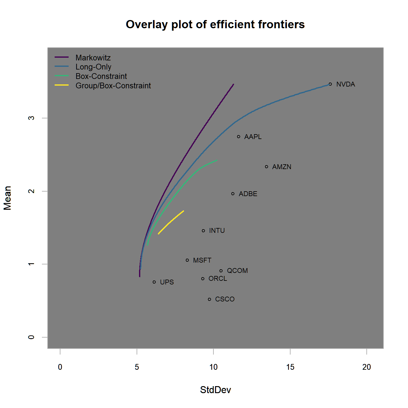
FIGURE 4.13: Efficient frontiers for all 4 previous examples (unconstrained, long-only, long-only with box constraints and long-only with box and group constraints).
Using this figure, we want to highlight several important facts about portfolio optimization:
- In the classical \(mu\)-\(sigma\)-diagram (aka ‘Mean-StdDev’ in the plots above) we find that less constrained efficient frontiers are positioned further to the north-west. In the language of portfolio optimization an asset or a portfolio is better than another if it lies further to the north-west and therefore dominates the other. In other words, it has either a lower risk for a given return level or a higher return for a given level of risk. All assets and portfolios, that are not dominated by any other asset or portfolio are called efficient, hence the efficient frontier as locus of all ‘most dominant’ portfolio allocations.
TTTTTTTTTTTTTTTTTTTTTTTTTTTTTTTTTTTTTTTTTTTTTTTTTTTTTTTTTTTTTTTTT
The obtained figure clearly shows us the impact of optimization constraints and objectives. This mainly can be summarized by two findings.
- The first finding relates to the preferred direction of a portfolio (or the efficient frontier itself) within the \(\mu\)-\(\sigma\) space.
It is the
north-westdirection which is preferred. Goingnorth-westimplies a higher return for the same risk, lower risk for same return or a combination of both. -
Second, the more restrictions applied in a mean-variance portfolio optimization, the more inefficient the efficient frontier becomes.
It is clearly visible, that the
Markowitz frontieris superior over theLong-Only frontierand theBox-Constrained frontiersince it lies relative in thenorth-westdirection and therefore dominates both from a mean-variance perspective. This is also indicated by the ex-ante Sharpe ratios. [TBD]
Notice that the efficient frontier comprises the upper (most north-westerly) bound for all individual assets as well as all possible sub-portfolios. Hence, with a given set of (i) assets, (ii) optimization constraints, and (iii) objectives, it is not possible to build a portfolio that reaches a region beyond the efficient frontier. Beside the differences, however, all three frontiers form relatively unrestricted optimization examples. In practice, portfolio managers most often are exposed to many more complex restrictions, such as box or group constraints.
4.3.2 Important mean-variance portfolios and efficient frontiers
In the following, we will step by step build up several different parts of the efficient frontier without (only investing in risky assets) and with (leading to two-fund separation and the Capital Allocation Line) the existence of the risk-free interest rate. We will step-by-step calculate:
- The global minimum variance portfolio (GMVP) defining the lower end of the efficient frontier
- The maximum return portfolio (MRP) defining the upper end of the efficient frontier
- Three target return portfolios (TR1-TR3) along the efficient frontier, where we select the target returns equally spaced between the GMVP and the MRP.
- The tangency portfolio (TPF) given the existence of a risk-free interest rate \(r_f\).
- Two maximum quadratic utility portfolios (MU1-MU2) for risk-aversion levels of \(\gamma=1\) and \(\gamma=8\) along the Capital Allocation Line, again assuming the existence of the risk-free interest rate \(r_f\).
In the case where the only constraint is a full-investment constraint, we directly minimize risk (without a target return constraint) to calculate the global minimum variance portfolio, solving (4.1) as \[\begin{equation} w_{MVP}=\frac{\Sigma^{-1}\mathbf{1}}{\mathbf{1}\Sigma^{-1}\mathbf{1}} \tag{4.3} \end{equation}\] where the denominator is necessary to have the weights sum to one and assure full investment. Solving (4.2) without the target risk constraint yields the global maximum return portfolio, \[\begin{equation} w_{MRT}=1_{max(\mu)}, \tag{4.4} \end{equation}\] where the weight is equal to \(1\) for the asset with the highest expected return \(\mu\) and \(0\) for all others.
The tangency portfolio, for a given risk free rate \(r_f\) can be found by maximizing the Sharpe Ratio \[\begin{align} & \underset{w}{\text{max}} & & \frac{w'\mu - r_f}{\sqrt{w'\Sigma w}}\\ &&& w'\mathbf{1}=1. \tag{4.5} \end{align}\] and yields as solution \[\begin{equation} w_{TP}=\frac{\Sigma^{-1}\left(\mu-r_f\cdot\mathbf{1}\right)}{\mathbf{1}\Sigma^{-1}\left(\mu-r_f\cdot\mathbf{1}\right)}, \tag{4.6} \end{equation}\] an equation that is similar to the one derived in (4.3) above.
For the target return portfolio we determine the target returns as \[\begin{equation} \mu_{Target,i}=\mu(MVP)+\frac{\mu(maxRet)-\mu(MVP)}{4}\Cdot i,\quad i\in\{1,2,3\} \tag{4.7} \end{equation}\] and a portfolio solution of …
ADD FORMULA FOR OPTIMAL TARGET RETURN
Last and least we need to specify a particular level of risk aversion to find the optimal quadratic utility portfolio along the capital allocation line (as all the portfolios on the CAL yield the same Sharpe ratio). For this we optimize quadratic utility \[\begin{equation} \underset{w}{\text{max }} w^{'} \mu - \frac{\gamma}{2} w^{'} \Sigma w \tag{4.8} \end{equation}\] and get as optimal complete portfolio, given the risk-free rate \(r_f\) as well as the tangency portfolio \(w_{TP}\) that yields Sharpe ratio \(SR_{TP}=\frac{\mu_{TP}}{\sigma_{TP}}\): \[\begin{equation} \dots \tag{4.9} \end{equation}\]
Thus, for each frontier specification we end up with seven portfolios for which we chart the optimal weights using chart.Weights() as well as their position in the \(\mu\)-\(\sigma\)-diagram using chart.RiskReward() which we overlay to the efficient frontier using par(new=TRUE).
4.3.2.1 The full-investment frontier
We start by defining three portfolio objects, where we add a full-investment constraint to all portfolios. For the maximum return portfolio, we only need to define the return objective. Similarly, for the global minimum variance portfolio, it is sufficient to define a variance objective. Adding a mean objective changes the optimization framework to a Maximum Quadratic Utility optimization, where - given a large enough risk-aversion parameter - under the full-investment constraint we will also end up with the most conservative portfoilio possible, which is the Minimum Variance Portfolio. We do this, because this allows us to extract the mean of the optimal portfolio using extractObjectiveMeasures() or alternatively using extractStats() for later use. We also optimize the tangency portfolio, where adding maxSR=TRUE changes the maximum quadratic utility framework to a Sharpe-ratio optimization. In a next step, we extract the means from the maximum return as well as the global minimum variance portfolios and define three target return portfolios via a target return constraint as well as a variance objective equally spaced between both returns. Last, we optimize two maximum quadratic utility portfolios with two levels of risk aversion: \(1\) and \(8\)27 where we relax the full investment constraint to allow for a selection of the optimal complete portfolio along the Capital Allocation line, thereby mixing the tangency portfolio with the risk-free interest rate28. Also note that we can directly specify one quadratic utility objective including the risk-aversion parameter, rather than specifying two mean and variance objectives.
# Minimum variance portfolio
M.spec.mvp <- pspec %>%
  add.constraint(type = "full_investment") %>%
  add.objective(type = "risk", name = "StdDev", risk_aversion=9999) %>%
  add.objective(type = "return", name = "mean")
# Tangency portfolio
M.spec.tp <- pspec %>%
  add.constraint(type = "full_investment") %>%
  add.objective(type = "risk", name = "StdDev") %>%
  add.objective(type = "return", name = "mean")
# Max return portfolio
M.spec.maxret <- pspec %>%
  add.constraint(type = "full_investment") %>%
  add.constraint(type = "box", min=0, max=1) %>%
  add.objective(type = "return", name = "mean")

# Optimize portfolios
M.tp <- optimize.portfolio(returns, M.spec.tp,
                           optimize_method = "ROI", maxSR=TRUE, trace = TRUE)
M.mvp <- optimize.portfolio(returns, M.spec.mvp,
                           optimize_method = "ROI", trace = TRUE)
M.maxret <- optimize.portfolio(returns, M.spec.maxret,
                           optimize_method = "ROI", trace = TRUE)

# Define target returns
M.maxret.mu <- unname(extractObjectiveMeasures(M.maxret)$mean)# Max ret
M.mvp.mu <- unname(extractObjectiveMeasures(M.mvp)$mean) # Min ret: MVP
ret.M <- M.mvp.mu+(1:3*(M.maxret.mu-M.mvp.mu)/4) # ret vector

# Target return portfolios
M.spec.ret <- pspec %>%
  add.constraint(type = "full_investment") %>%
  add.objective(type = "risk", name = "StdDev")
M.spec.ret1 <- M.spec.ret %>%
  add.constraint(type="return", return_target=ret.M[1])
M.spec.ret2 <- M.spec.ret %>%
  add.constraint(type="return", return_target=ret.M[2])
M.spec.ret3 <- M.spec.ret %>%
  add.constraint(type="return", return_target=ret.M[3])

# Quadratic utility portfolios
M.spec.util1 <- pspec %>%
  add.constraint(type = "weight_sum", min=0, max=2) %>%
  add.objective(type = "quadratic_utility", name = "var", risk_aversion=1/100)
M.spec.util2 <- pspec %>%
  add.constraint(type = "weight_sum", min=0, max=1) %>%
  add.objective(type = "quadratic_utility", name = "var", risk_aversion=8/100)

# optimize portfolios
M.ret1 <- optimize.portfolio(returns, M.spec.ret1,
                             optimize_method = "ROI", trace = TRUE)
M.ret2 <- optimize.portfolio(returns, M.spec.ret2,
                             optimize_method = "ROI", trace = TRUE)
M.ret3 <- optimize.portfolio(returns, M.spec.ret3,
                             optimize_method = "ROI", trace = TRUE)
M.util1 <- optimize.portfolio(returns, M.spec.util1,
                              optimize_method = "ROI", trace = TRUE)
M.util2 <- optimize.portfolio(returns, M.spec.util2,
                              optimize_method = "ROI", trace = TRUE)
In a next step, we make use of several more complex plotting procedures in R to overlay the efficient frontier plot that includes the individual assets with a plot that includes all the optimized portfolios. For this we first need to define a list of optimize.portfolio() objects, so that we can plot all portfolios with one call to chart.RiskReward() using combine.optimizations().
# create List of portfolios objects
M.list <- list(M.mvp,M.ret1,M.ret2,M.ret3,M.util1,M.util2,M.maxret)
names(M.list) <- c("MVP","TRet1","Tret2","Tret3","Util1","Util2","MaxRet")

chart.EfficientFrontier(M.tp, match.col = "StdDev", n.portfolios = 10,
                        xlim = c(0,20), ylim = c(0,5),
                        tangent.line = TRUE, rf=0, type="line",
                        chart.assets = TRUE, labels.assets = TRUE)
par(new = TRUE)
chart.RiskReward(combine.optimizations(M.list),
                 neighbors=10, risk.col="StdDev",
                        chart.assets = FALSE, labels.assets = TRUE,
                 xlim = c(0,20), ylim = c(0,5))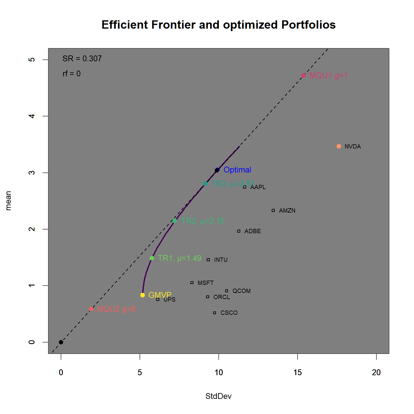
FIGURE 4.14: Efficient frontier with an optimized portfolio overlay.
In 4.14 we find the minimum variance, as well as the target return and the tangency portfolios to be allocated on the efficient frontier in ascending order. The efficient frontier clearly surpasses the maximum return portfolio (100% investment in Nvidia), as we allow - in this most general setting - for the possibility to short sell assets. The maximum quadratic utility portfolios are all allocated on the Capital Allocation Line (which by definition is the new efficient frontier once we allow for the existence of a risk-free asset) on both sides of the tangency portfolios. In 4.15 we additionally observe the portfolio weights (stacked by Asset and Portfolio). We immediately observe, that the portfolios with higher target returns do more heavily adhere to short-selling. Additionally the two maximum utility portfolios have weight sums different from one (and therefore subject to some form of leverage). Except for Qualcom (QCOM) all asset are subject to some form of investment. We conclude, that QCOM (as it is anyway dominated by Microsoft or Oracle) is not even a good applicant for diversification. Note, that the relation between asset weights is exactly the same for the two maximum utility as wella s the tangency portfolio!
# create List of portfolios objects
M.list <- list(M.util2,M.mvp,M.ret1,M.ret2,M.ret3,M.tp,M.util1,M.maxret)
names(M.list) <- c("Util2","MVP","TRet1","Tret2","Tret3","TP","Util1","MaxRet")

chart.Weights(combine.optimizations(M.list), plot.type = "barplot",
              main="Weights (stacked by Asset)"))
chart.StackedBar(w=extractWeights(combine.optimizations(M.list)),
                 main="Weights (stacked by Portfolio)")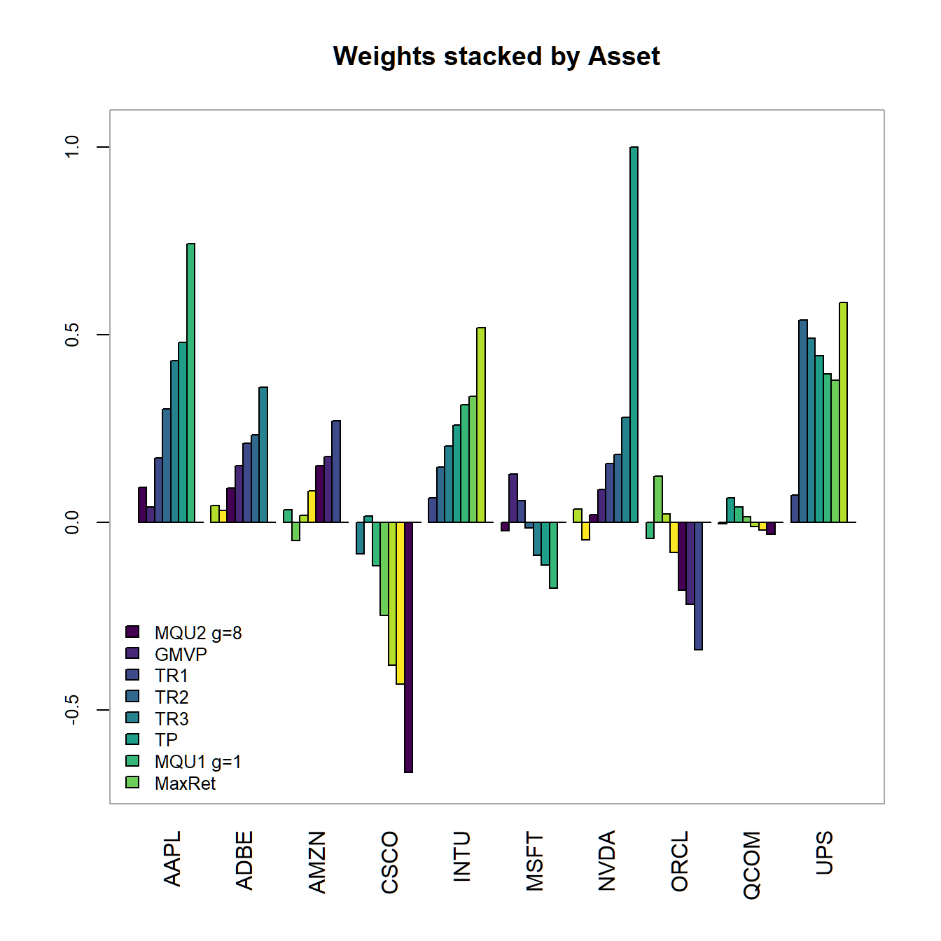
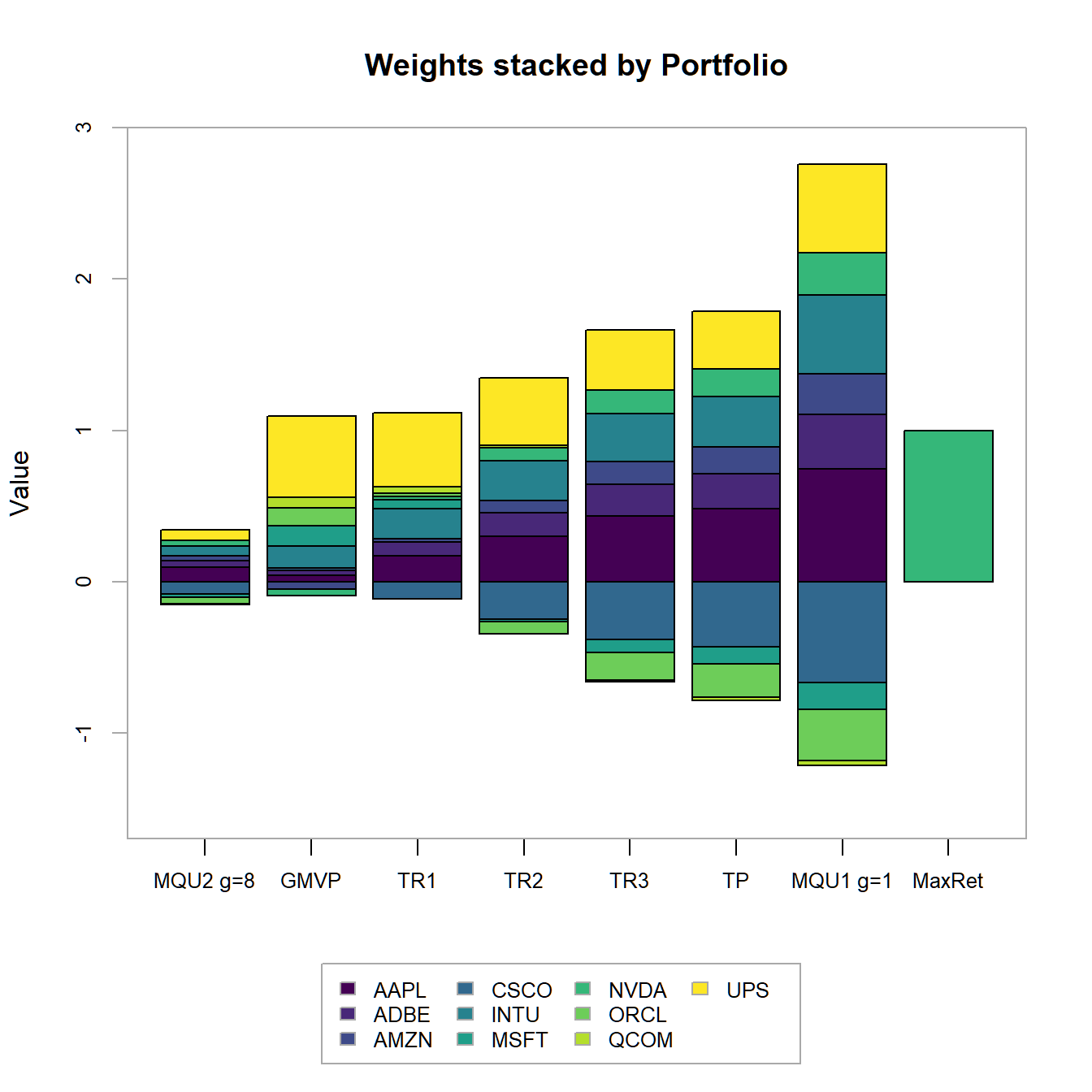
FIGURE 4.15: Portfolio weights stacked by portfolio for all optimized portfolios.
4.3.2.2 The long-only frontier
In a next step, we add constraints to observer their impact on the different portfolios.
pspecLO <- pspec %>%
  add.constraint(type = "long_only")
# Minimum variance portfolio
LO.spec.mvp <- pspecLO %>%
  add.constraint(type = "full_investment") %>%
  add.objective(type = "risk", name = "StdDev", risk_aversion=9999) %>%
  add.objective(type = "return", name = "mean")
# Tangency portfolio
LO.spec.tp <- pspecLO %>%
  add.constraint(type = "full_investment") %>%
  add.objective(type = "risk", name = "StdDev") %>%
  add.objective(type = "return", name = "mean")
# Max return portfolio
LO.spec.maxret <- pspecLO %>%
  add.constraint(type = "full_investment") %>%
  add.constraint(type = "box", min=0, max=1) %>%
  add.objective(type = "return", name = "mean")

# Optimize portfolios
LO.tp <- optimize.portfolio(returns, LO.spec.tp,
                            optimize_method = "ROI", maxSR=TRUE, trace = TRUE)
LO.mvp <- optimize.portfolio(returns, LO.spec.mvp,
                            optimize_method = "ROI", trace = TRUE)
LO.maxret <- optimize.portfolio(returns, LO.spec.maxret,
                            optimize_method = "ROI", trace = TRUE)

# Define target returns
LO.maxret.mu <- unname(extractObjectiveMeasures(LO.maxret)$mean)# Max ret
LO.mvp.mu <- unname(extractObjectiveMeasures(LO.mvp)$mean) # Min ret: MVP
ret.M <- LO.mvp.mu+(1:3*(LO.maxret.mu-LO.mvp.mu)/4) # ret vector

# Target return portfolios
LO.spec.ret <- pspecLO %>%
  add.constraint(type = "full_investment") %>%
  add.objective(type = "risk", name = "StdDev")
LO.spec.ret1 <- LO.spec.ret %>%
  add.constraint(type="return", return_target=ret.M[1])
LO.spec.ret2 <- LO.spec.ret %>%
  add.constraint(type="return", return_target=ret.M[2])
LO.spec.ret3 <- LO.spec.ret %>%
  add.constraint(type="return", return_target=ret.M[3])

# Quadratic utility portfolios
LO.spec.util1 <- pspecLO %>%
  add.constraint(type = "weight_sum", min=0, max=2) %>%
  add.objective(type = "quadratic_utility", name = "var", risk_aversion=1/100)
LO.spec.util2 <- pspecLO %>%
  add.constraint(type = "weight_sum", min=0, max=1) %>%
  add.objective(type = "quadratic_utility", name = "var", risk_aversion=8/100)

# optimize portfolios
LO.ret1 <- optimize.portfolio(returns, LO.spec.ret1,
                              optimize_method = "ROI", trace = TRUE)
LO.ret2 <- optimize.portfolio(returns, LO.spec.ret2,
                              optimize_method = "ROI", trace = TRUE)
LO.ret3 <- optimize.portfolio(returns, LO.spec.ret3,
                              optimize_method = "ROI", trace = TRUE)
LO.util1 <- optimize.portfolio(returns, LO.spec.util1,
                              optimize_method = "ROI", trace = TRUE)
LO.util2 <- optimize.portfolio(returns, LO.spec.util2,
                              optimize_method = "ROI", trace = TRUE)
# create List of portfolios objects
LO.list <- list(LO.mvp,LO.ret1,LO.ret2,LO.ret3,LO.util1,LO.util2,LO.maxret)
names(LO.list) <- c("MVP","TRet1","Tret2","Tret3","Util1","Util2","MaxRet")

chart.EfficientFrontier(LO.tp, match.col = "StdDev", n.portfolios = 10,
                        xlim = c(0,20), ylim = c(0,5),
                        tangent.line = TRUE, rf=0, type="line",
                        chart.assets = TRUE, labels.assets = TRUE)
par(new = TRUE)
chart.RiskReward(combine.optimizations(LO.list),
                 neighbors=10, risk.col="StdDev",
                        chart.assets = FALSE, labels.assets = TRUE,
                 xlim = c(0,20), ylim = c(0,5))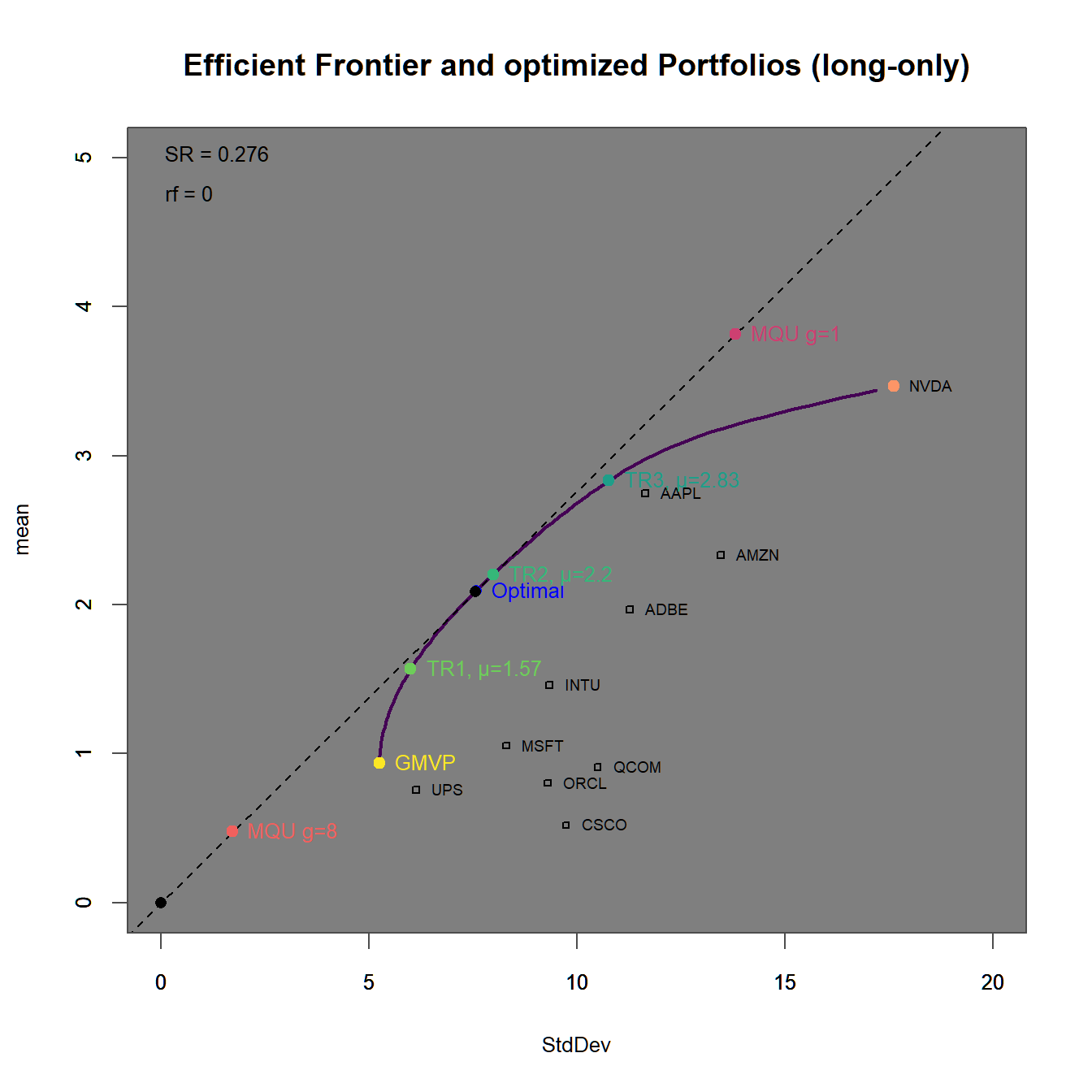
FIGURE 4.16: Efficient frontier with an optimized portfolio overlay.
In 4.16 we find
In 4.17
We immediately observe, that the portfolios with higher target returns do more heavily adhere to short-selling. Additionally the two maximum utility portfolios have weight sums different from one (and therefore subject to some form of leverage).
# create List of portfolios objects
LO.list <- list(LO.util2,LO.mvp,LO.ret1,LO.ret2,LO.ret3,LO.tp,LO.util1,LO.maxret)
names(LO.list) <- c("Util2","MVP","TRet1","Tret2","Tret3","TP","Util1","MaxRet")

chart.Weights(combine.optimizations(LO.list), plot.type = "barplot",
              main="Weights stacked by Asset (long-only)"))
chart.StackedBar(w=extractWeights(combine.optimizations(LO.list)),
                 main="Weights stacked by Portfolio (long-only))")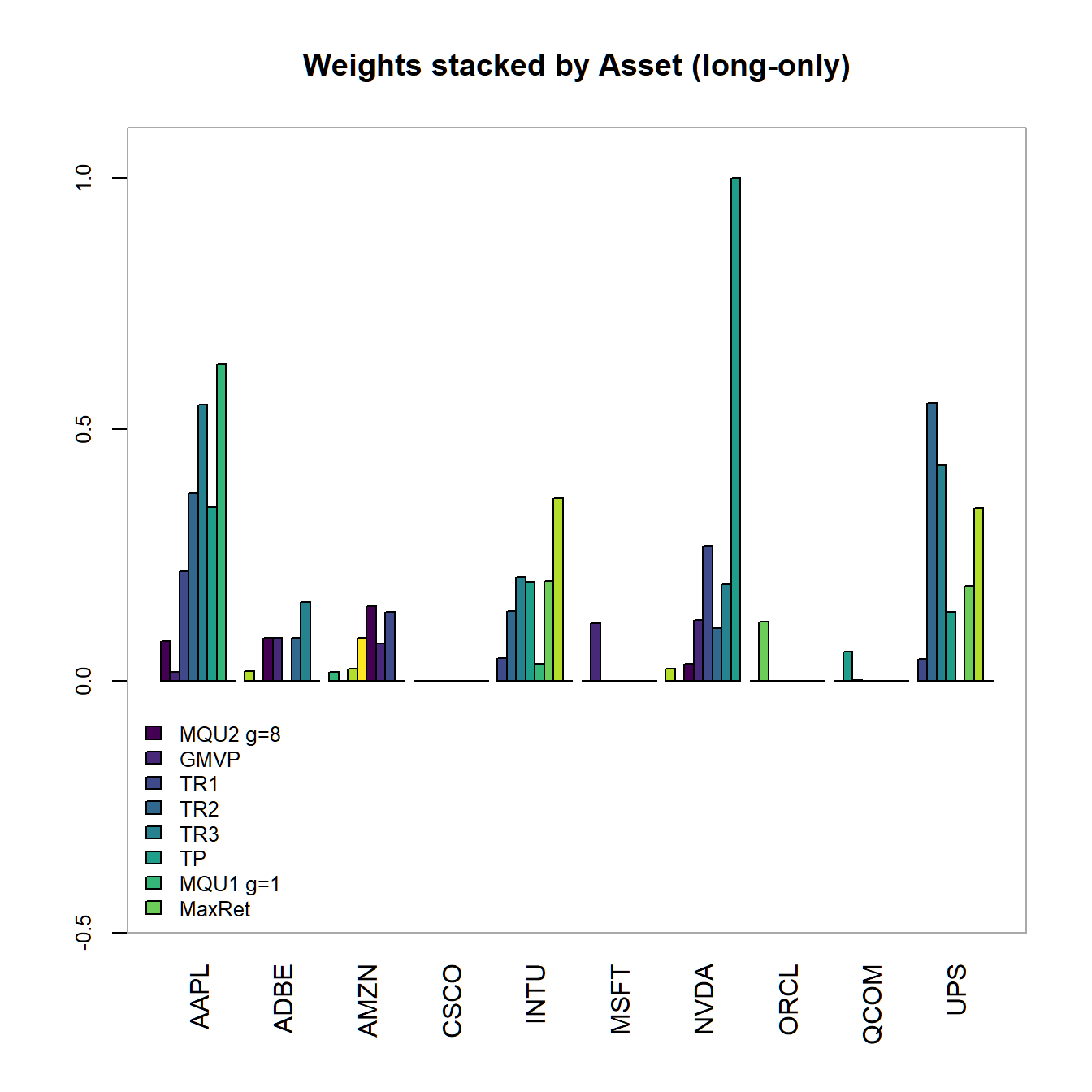
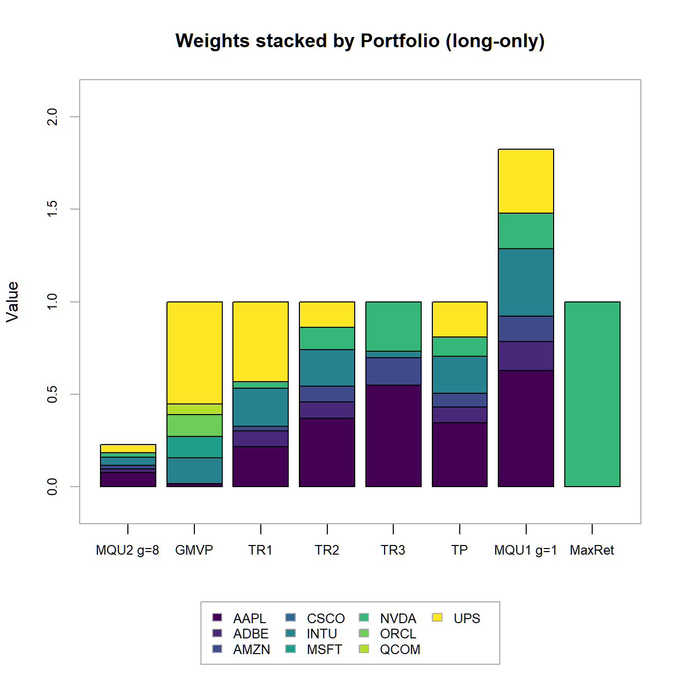
FIGURE 4.17: Portfolio weights stacked by portfolio for all optimized long-only portfolios.
Main findings: - Sum of weights adds up to one - But, we observe zero weights in certain assets - How to solve this issue? -> Impose box-constraints
4.3.2.3 Box constraints and the long-only frontier
In a next step, we add constraints to observer their impact on the different portfolios.
pspecBLO <- pspecLO %>%
  add.constraint(type = "box", name ="x", min=0.05, max=0.4)
# Minimum variance portfolio
BLO.spec.mvp <- pspecBLO %>%
  add.constraint(type = "full_investment") %>%
  add.objective(type = "risk", name = "StdDev", risk_aversion=9999) %>%
  add.objective(type = "return", name = "mean")
# Tangency portfolio
BLO.spec.tp <- pspecBLO %>%
  add.constraint(type = "full_investment") %>%
  add.objective(type = "risk", name = "StdDev") %>%
  add.objective(type = "return", name = "mean")
# Max return portfolio
BLO.spec.maxret <- pspecBLO %>%
  add.constraint(type = "full_investment") %>%
  add.objective(type = "return", name = "mean")

# Optimize portfolios
BLO.tp <- optimize.portfolio(returns, BLO.spec.tp,
                             optimize_method = "ROI", maxSR=TRUE, trace = TRUE)
BLO.mvp <- optimize.portfolio(returns, BLO.spec.mvp,
                             optimize_method = "ROI", trace = TRUE)
BLO.maxret <- optimize.portfolio(returns, BLO.spec.maxret,
                             optimize_method = "ROI", trace = TRUE)

# Define target returns
BLO.maxret.mu <- unname(extractObjectiveMeasures(BLO.maxret)$mean)# Max ret
BLO.mvp.mu <- unname(extractObjectiveMeasures(BLO.mvp)$mean) # Min ret: MVP
ret.M <- BLO.mvp.mu+(1:3*(BLO.maxret.mu-BLO.mvp.mu)/4) # ret vector

# Target return portfolios
BLO.spec.ret <- pspecBLO %>%
  add.constraint(type = "full_investment") %>%
  add.objective(type = "risk", name = "StdDev")
BLO.spec.ret1 <- BLO.spec.ret %>%
  add.constraint(type="return", return_target=ret.M[1])
BLO.spec.ret2 <- BLO.spec.ret %>%
  add.constraint(type="return", return_target=ret.M[2])
BLO.spec.ret3 <- BLO.spec.ret %>%
  add.constraint(type="return", return_target=ret.M[3])

# Quadratic utility portfolios
BLO.spec.util1 <- pspecBLO %>%
  add.constraint(type = "weight_sum", min=0, max=2) %>%
  add.objective(type = "quadratic_utility", name = "var", risk_aversion=1/100)
BLO.spec.util2 <- pspecBLO %>%
  add.constraint(type = "weight_sum", min=0, max=1) %>%
  add.objective(type = "quadratic_utility", name = "var", risk_aversion=8/100)

# optimize portfolios
BLO.ret1 <- optimize.portfolio(returns, BLO.spec.ret1,
                               optimize_method = "ROI", trace = TRUE)
BLO.ret2 <- optimize.portfolio(returns, BLO.spec.ret2,
                               optimize_method = "ROI", trace = TRUE)
BLO.ret3 <- optimize.portfolio(returns, BLO.spec.ret3,
                               optimize_method = "ROI", trace = TRUE)
BLO.util1 <- optimize.portfolio(returns, BLO.spec.util1,
                               optimize_method = "ROI", trace = TRUE)
BLO.util2 <- optimize.portfolio(returns, BLO.spec.util2,
                               optimize_method = "ROI", trace = TRUE)
# create List of portfolios objects
BLO.list <- list(BLO.mvp,BLO.ret1,BLO.ret2,BLO.ret3,BLO.util1,BLO.util2,BLO.maxret)
names(Mlist) <- c("MVP","TRet1","Tret2","Tret3","Util1","Util2","MaxRet")

chart.EfficientFrontier(BLO.tp, match.col = "StdDev", n.portfolios = 10,
                        xlim = c(0,20), ylim = c(0,5),
                        tangent.line = TRUE, rf=0, type="line",
                        chart.assets = TRUE, labels.assets = TRUE)
par(new = TRUE)
chart.RiskReward(combine.optimizations(BLO.list),
                 neighbors=10, risk.col="StdDev",
                        chart.assets = FALSE, labels.assets = TRUE,
                 xlim = c(0,20), ylim = c(0,5))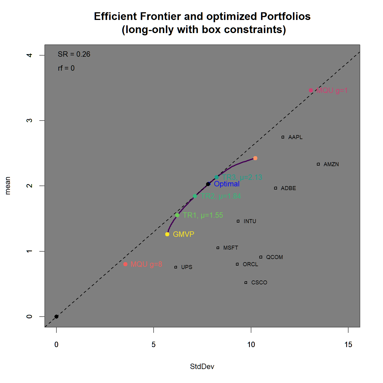
FIGURE 4.18: Efficient frontier with an optimized portfolio overlay.
In 4.18 we find In 4.19 we find
We immediately observe, that the portfolios with higher target returns do more heavily adhere to short-selling. Additionally the two maximum utility portfolios have weight sums different from one (and therefore subject to some form of leverage).
# create List of portfolios objects
BLO.list <- list(BLO.util2,BLO.mvp,BLO.ret1,BLO.ret2,BLO.ret3,
                 BLO.tp,BLO.util1,BLO.maxret)
names(BLO.list) <- c("Util2","MVP","TRet1","Tret2","Tret3",
                     "TP","Util1","MaxRet")

chart.Weights(combine.optimizations(BLO.list), plot.type = "barplot",
              main="Weights stacked by Asset\n
              (long-only and box constraints)"))
chart.StackedBar(w=extractWeights(combine.optimizations(BLO.list)),
                 main="Weights stacked by Portfolio\n
                 (long-only and box constraints)")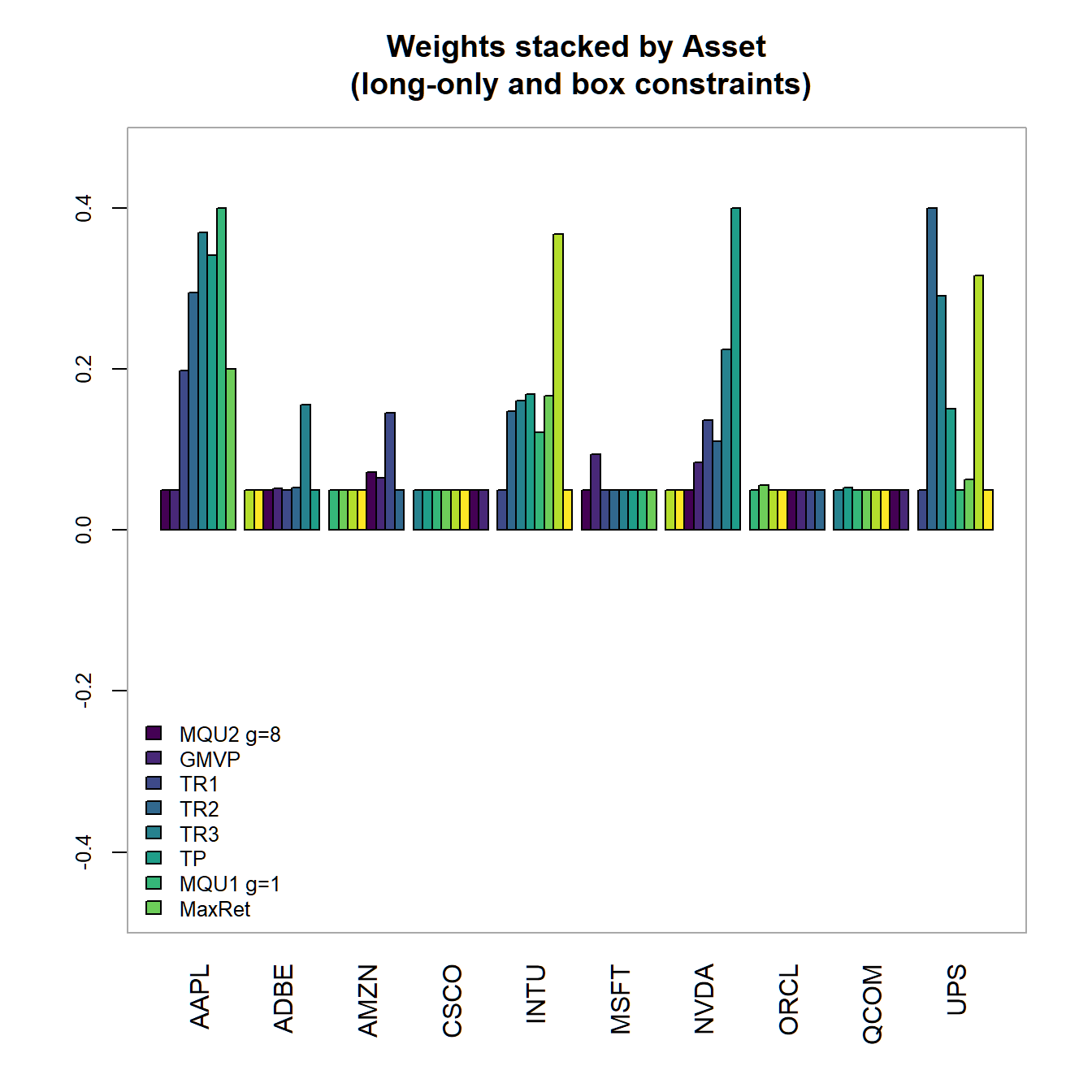
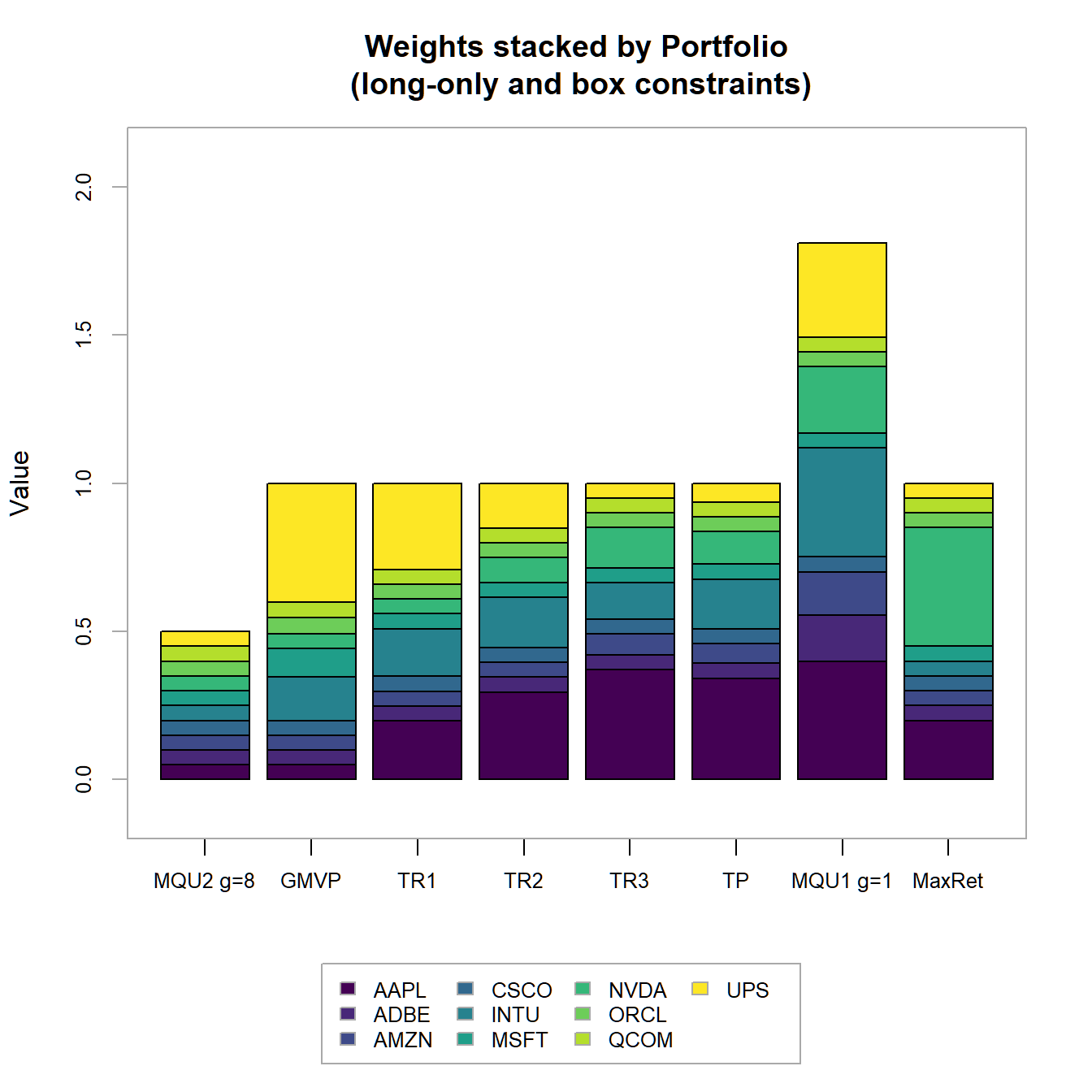
FIGURE 4.19: Portfolio weights stacked by portfolio for all optimized long-only portfolios.
4.3.2.4 Group & box constraints and the long-only frontier
In a next step, we add constraints to observer their impact on the different portfolios.
pspecGBLO <- pspecBLO %>%
  add.constraint(type="group",
                 # list of vectors specifying the groups of the assets
                 groups=list(pspec$category_labels$`Information Technology`,
                             pspec$category_labels$`Consumer Discretionary`,
                             pspec$category_labels$`Industrials`),
                 group_min=c(0.1, 0.15,0.1),
                 group_max=c(0.4, 0.55,0.4),
                 group_labels=pspec$category_labels)
# Minimum variance portfolio
GBLO.spec.mvp <- pspecGBLO %>%
  add.constraint(type = "full_investment") %>%
  add.objective(type = "risk", name = "StdDev", risk_aversion=9999) %>%
  add.objective(type = "return", name = "mean")
# Tangency portfolio
GBLO.spec.tp <- pspecGBLO %>%
  add.constraint(type = "full_investment") %>%
  add.objective(type = "risk", name = "StdDev") %>%
  add.objective(type = "return", name = "mean")
# Max return portfolio
GBLO.spec.maxret <- pspecGBLO %>%
  add.constraint(type = "full_investment") %>%
  add.objective(type = "return", name = "mean")

# Optimize portfolios
GBLO.tp <- optimize.portfolio(returns, GBLO.spec.tp,
                              optimize_method = "ROI", maxSR=TRUE, trace = TRUE)
GBLO.mvp <- optimize.portfolio(returns, GBLO.spec.mvp,
                              optimize_method = "ROI", trace = TRUE)
GBLO.maxret <- optimize.portfolio(returns, GBLO.spec.maxret,
                              optimize_method = "ROI", trace = TRUE)

# Define target returns
GBLO.maxret.mu <- unname(extractObjectiveMeasures(GBLO.maxret)$mean)# Max ret
GBLO.mvp.mu <- unname(extractObjectiveMeasures(GBLO.mvp)$mean) # Min ret: MVP
ret.M <- GBLO.mvp.mu+(1:3*(GBLO.maxret.mu-GBLO.mvp.mu)/4) # ret vector

# Target return portfolios
GBLO.spec.ret <- pspecGBLO %>%
  add.constraint(type = "full_investment") %>%
  add.objective(type = "risk", name = "StdDev")
GBLO.spec.ret1 <- GBLO.spec.ret %>%
  add.constraint(type="return", return_target=ret.M[1])
GBLO.spec.ret2 <- GBLO.spec.ret %>%
  add.constraint(type="return", return_target=ret.M[2])
GBLO.spec.ret3 <- GBLO.spec.ret %>%
  add.constraint(type="return", return_target=ret.M[3])

# Quadratic utility portfolios
GBLO.spec.util1 <- pspecGBLO %>%
  add.constraint(type = "weight_sum", min=0, max=2) %>%
  add.objective(type = "quadratic_utility", name = "var", risk_aversion=1/100)
GBLO.spec.util2 <- pspecGBLO %>%
  add.constraint(type = "weight_sum", min=0, max=1) %>%
  add.objective(type = "quadratic_utility", name = "var", risk_aversion=8/100)

# optimize portfolios
GBLO.ret1 <- optimize.portfolio(returns, GBLO.spec.ret1,
                                optimize_method = "ROI", trace = TRUE)
GBLO.ret2 <- optimize.portfolio(returns, GBLO.spec.ret2,
                                optimize_method = "ROI", trace = TRUE)
GBLO.ret3 <- optimize.portfolio(returns, GBLO.spec.ret3,
                                optimize_method = "ROI", trace = TRUE)
GBLO.util1 <- optimize.portfolio(returns, GBLO.spec.util1,
                                optimize_method = "ROI", trace = TRUE)
GBLO.util2 <- optimize.portfolio(returns, GBLO.spec.util2,
                                optimize_method = "ROI", trace = TRUE)
# create List of portfolios objects
GBLO.list <- list(GBLO.mvp,GBLO.ret1,GBLO.ret2,GBLO.ret3,GBLO.util1,GBLO.util2,GBLO.maxret)
names(Mlist) <- c("MVP","TRet1","Tret2","Tret3","Util1","Util2","MaxRet")

chart.EfficientFrontier(GBLO.tp, match.col = "StdDev", n.portfolios = 10,
                        xlim = c(0,20), ylim = c(0,5),
                        tangent.line = TRUE, rf=0, type="line",
                        chart.assets = TRUE, labels.assets = TRUE)
par(new = TRUE)
chart.RiskReward(combine.optimizations(GBLO.list),
                 neighbors=10, risk.col="StdDev",
                        chart.assets = FALSE, labels.assets = TRUE,
                 xlim = c(0,20), ylim = c(0,5))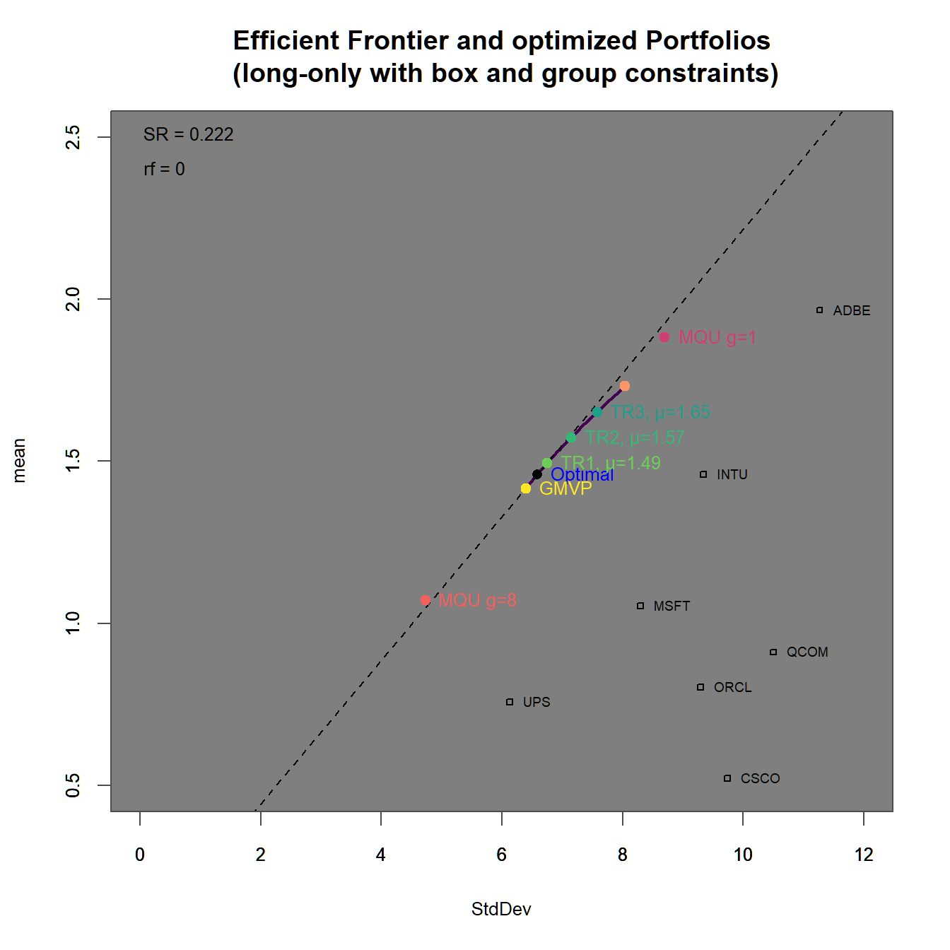
FIGURE 4.20: Efficient frontier with an optimized portfolio overlay (box ).
In 4.20 we find
In 4.21 we find
We immediately observe, that the portfolios with higher target returns do more heavily adhere to short-selling. Additionally the two maximum utility portfolios have weight sums different from one (and therefore subject to some form of leverage).
# create List of portfolios objects
GBLO.list <- list(GBLO.util2,GBLO.mvp,GBLO.ret1,GBLO.ret2,GBLO.ret3,
                  GBLO.tp,GBLO.util1,GBLO.maxret)
names(GBLO.list) <- c("Util2","MVP","TRet1","Tret2","Tret3",
                      "TP","Util1","MaxRet")

chart.Weights(combine.optimizations(GBLO.list), plot.type = "barplot",
              main="Weights stacked by Asset\n
              (long-only, box and group constraints)"))
chart.StackedBar(w=extractWeights(combine.optimizations(GBLO.list)),
                 main="Weights stacked by Portfolio\n
                 (long-only, box and group constraints)")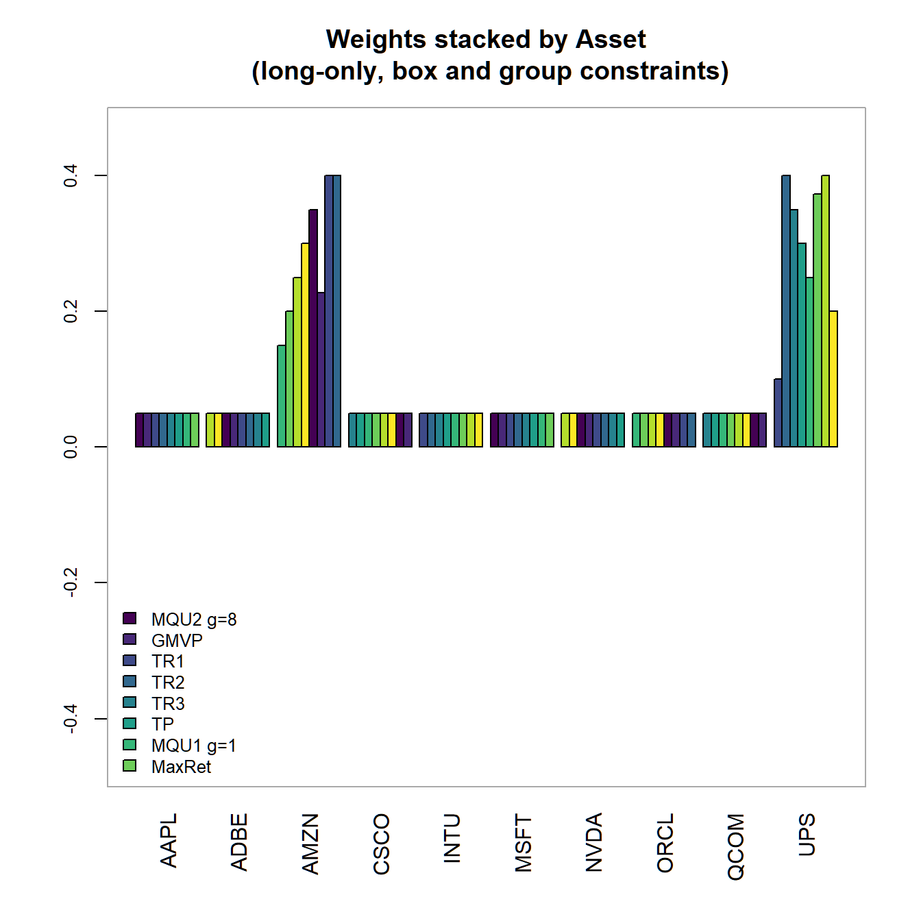
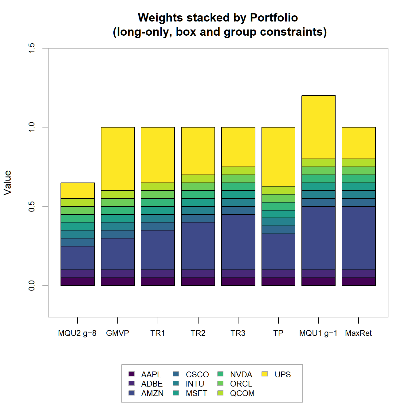
FIGURE 4.21: Portfolio weights stacked by portfolio for all optimized long-only portfolios with box and group constraints.